Audio Aliasing Visualization

import numpy as np
import matplotlib.pyplot as plt
from scipy.fft import fft
from IPython.display import Audio

1. Create a high-frequency sinusoid

SR = 44100  # Sampling rate for audio playback
f = 4000    # Frequency of the sinusoid
T = 1       # Duration in seconds
t = np.linspace(0, T, int(SR * T), endpoint=False) # Time vector
x = np.sin(2 * np.pi * f * t) # Sinusoid

2. Plot the time-domain signal

plt.figure(figsize=(12, 4))
plt.plot(t[:400], x[:400])
plt.title('Original High-Frequency Signal (Time Domain)')
plt.xlabel('Time (s)')
plt.ylabel('Amplitude')
plt.grid(True)
plt.show()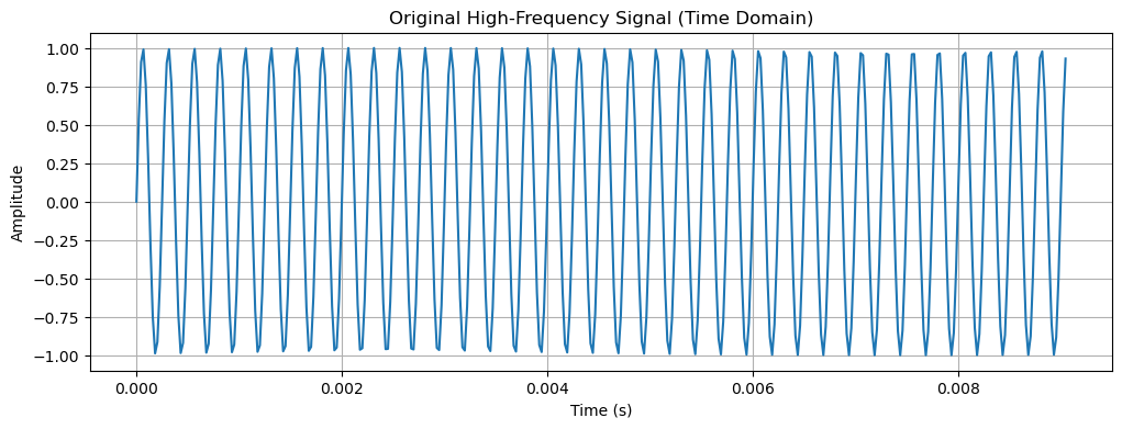

3. Play the audio of the original signal

Audio(x, rate=SR)

4. Plot the FFT (frequency-domain) of the original signal

N = len(x)
X = fft(x)
freq = np.fft.fftfreq(N, 1/SR)
plt.figure(figsize=(12, 4))
plt.plot(freq[:N//2], np.abs(X)[:N//2])
plt.title('Original Signal (Frequency Domain)')
plt.xlabel('Frequency (Hz)')
plt.ylabel('Magnitude')
plt.grid(True)
plt.show()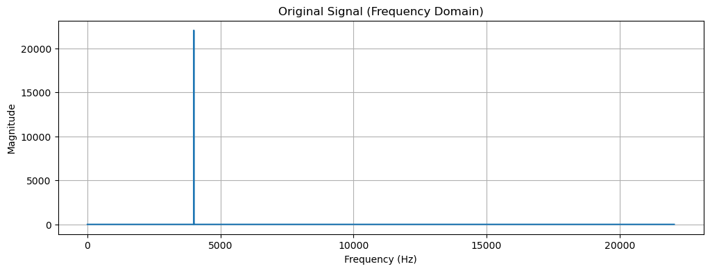

5. Resample the sinusoid using a sampling frequency that violates the Nyquist theorem

SR_low = 5000 # New sampling rate (less than 2*f)
t_low = np.linspace(0, T, int(SR_low * T), endpoint=False)
x_low = np.sin(2 * np.pi * f * t_low)

6. Plot the sampled points (the sampling signal)

plt.figure(figsize=(12, 4))
plt.plot(t[:400], x[:400], label='Original Signal')
plt.stem(t_low[:20], x_low[:20], 'r', markerfmt='ro', basefmt=' ', label='Sampled Points')
plt.title('Original Signal with Low-Rate Sampling Points')
plt.xlabel('Time (s)')
plt.ylabel('Amplitude')
plt.legend()
plt.grid(True)
plt.show()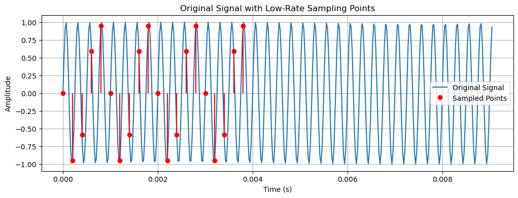

7. Plot the reconstructed (resampled) signal

plt.figure(figsize=(12, 4))
# plt.plot(t_low, x_low)
plt.plot(t_low[:50], x_low[:50])
plt.title('Reconstructed Signal from Low-Rate Sampling (Aliased)')
plt.xlabel('Time (s)')
plt.ylabel('Amplitude')
plt.grid(True)
plt.show()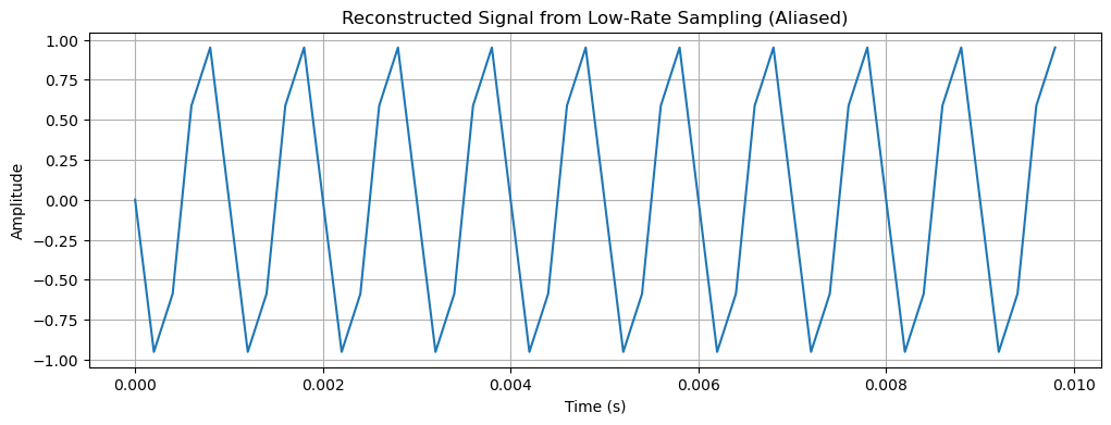

8. Play the audio of the resampled signal

Audio(x_low, rate=SR_low)

9. Plot the FFT of the resampled signal

N_low = len(x_low)
X_low = fft(x_low)
freq_low = np.fft.fftfreq(N_low, 1/SR_low)
plt.figure(figsize=(12, 4))
plt.plot(freq_low[:N_low//2], np.abs(X_low)[:N_low//2])
plt.title('Aliased Signal (Frequency Domain)')
plt.xlabel('Frequency (Hz)')
plt.ylabel('Magnitude')
plt.grid(True)
plt.show()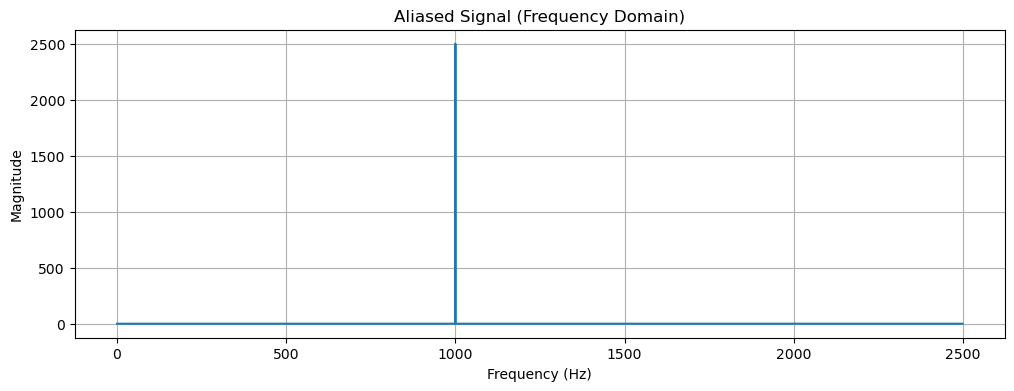

10. Resample the original sinusoid using a sampling frequency that satisfies the Nyquist theorem

SR_high = 10000 # New sampling rate (greater than 2*f)
t_high = np.linspace(0, T, int(SR_high * T), endpoint=False)
x_high = np.sin(2 * np.pi * f * t_high)

11. Plot the sampled points for this valid sampling

plt.figure(figsize=(12, 4))
plt.plot(t[:400], x[:400], label='Original Signal')
plt.stem(t_high[:40], x_high[:40], 'g', markerfmt='go', basefmt=' ', label='Sampled Points')
plt.title('Original Signal with High-Rate Sampling Points')
plt.xlabel('Time (s)')
plt.ylabel('Amplitude')
plt.legend()
plt.grid(True)
plt.show()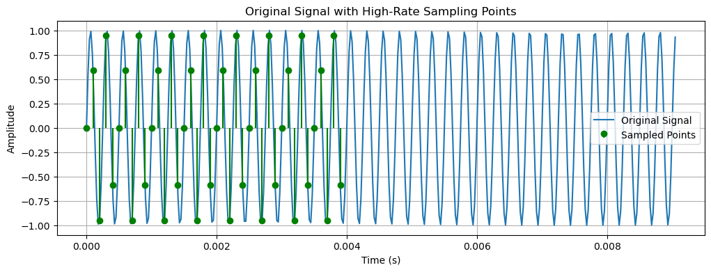

12. Plot the reconstructed (resampled) signal

plt.figure(figsize=(12, 4))
# plt.plot(t_high, x_high)
plt.plot(t_high[:100], x_high[:100])
plt.title('Reconstructed Signal from High-Rate Sampling')
plt.xlabel('Time (s)')
plt.ylabel('Amplitude')
plt.grid(True)
plt.show()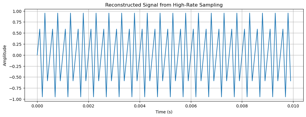

13. Play the audio of this correctly resampled signal

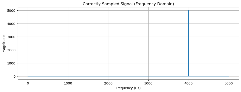
Audio(x_high, rate=SR_high)

14. Plot the FFT of the correctly resampled signal

N_high = len(x_high)
X_high = fft(x_high)
freq_high = np.fft.fftfreq(N_high, 1/SR_high)
plt.figure(figsize=(12, 4))
plt.plot(freq_high[:N_high//2], np.abs(X_high)[:N_high//2])
plt.title('Correctly Sampled Signal (Frequency Domain)')
plt.xlabel('Frequency (Hz)')
plt.ylabel('Magnitude')
plt.grid(True)
plt.show()