Signals and Systems
7.3 Undersampling, Aliasing, and Digital Signal Processing Fundamentals
Introduction: The Importance of Sampling
- Connecting Worlds: Sampling is the bridge between continuous-time (analog) signals and discrete-time (digital) signals.
- Digital Advantage: Allows us to process analog signals using powerful and flexible digital systems (computers, microcontrollers, DSPs).
- Core Concept: How do we represent a continuous signal with a finite set of discrete values?
- Reconstruction: How do we get the original continuous signal back from its samples?
- The Sampling Theorem: The theoretical foundation for perfect reconstruction.
Undersampling: The Effect of Aliasing
- Definition: Aliasing occurs when the sampling frequency \(\omega_s\) is less than twice the highest frequency \(\omega_M\) in the signal ($ _s < 2_M $).
- Consequence: The spectral replicas of the original signal \(X(j\omega)\) in the sampled signal’s spectrum \(X_p(j\omega)\) overlap.
- This overlap means the original signal’s spectrum is no longer recoverable by lowpass filtering.
- Time Domain: While the reconstructed signal \(x_r(t)\) will still match the original signal \(x(t)\) at the sampling instants (\(x_r(nT) = x(nT)\)), it will not be equal to \(x(t)\) between samples.
Aliasing is generally undesirable!
It introduces distortion where higher frequencies in the original signal are indistinguishable from lower frequencies after sampling, making perfect reconstruction impossible.
Aliasing: Time Domain Impact & Phase Reversal
- Time Domain Visualization: The lowpass filter, when aliasing occurs, attempts to fit a sinusoid of frequency less than \(\omega_s/2\) to the sampled points.
- This results in a reconstructed signal that has a different frequency than the original.
- Phase Reversal: For \(x(t) = \cos(\omega_0 t + \phi)\), aliasing can also cause a phase reversal.
- When \(\omega_s/2 < \omega_0 < \omega_s\), the reconstructed signal might be \(x_r(t) = \cos((\omega_s - \omega_0)t - \phi)\).
- The sign of the phase \(\phi\) is reversed.

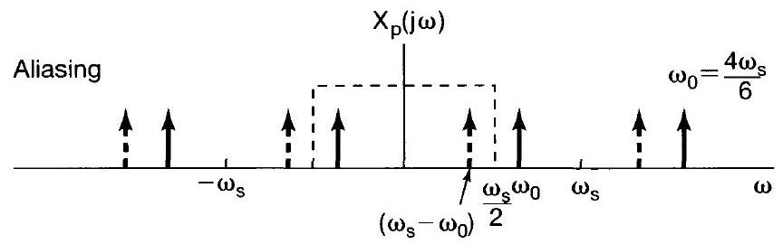
Figure 7.16 (c) Aliasing with ω0 = 4ωs/6: Original signal (solid), samples, and reconstructed signal (dashed) showing aliasing.
The Nyquist-Shannon Theorem requirement is strictly \(\omega_s > 2\omega_M\).
Sampling exactly at \(2\omega_M\) is not sufficient.
Example 7.1:
- \(x(t) = \cos((\omega_s/2)t + \phi)\) sampled at \(\omega_s\).
- Reconstructed: \(x_r(t) = (\cos \phi) \cos((\omega_s/2)t)\).
- Perfect reconstruction only if \(\phi = 0\).
- If \(x(t) = \sin((\omega_s/2)t)\) (\(\phi = -\pi/2\)), then \(x_r(t) = 0\). Samples are all zero!
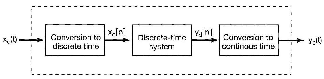
Equivalent Continuous-Time System
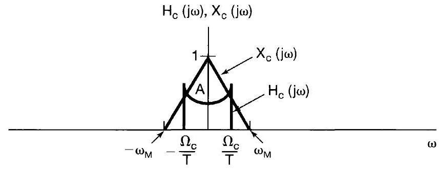
Application: Digital Differentiator
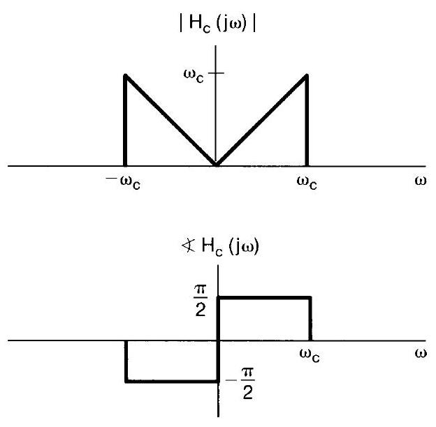
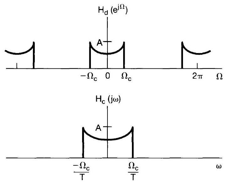
Ideal \(H_c(j\omega)\)
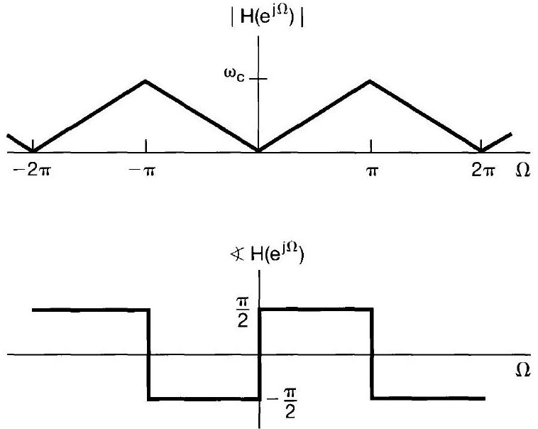
Corresponding \(H_d(e^{j\Omega})\)
Application: Half-Sample Delay
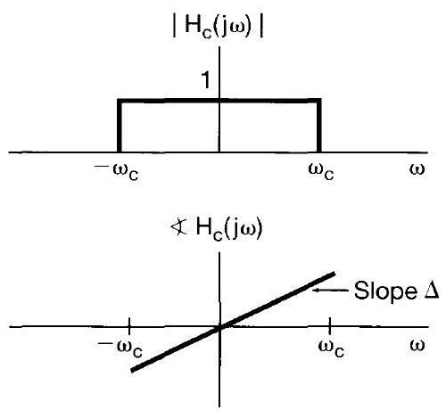
Ideal \(H_c(j\omega)\)
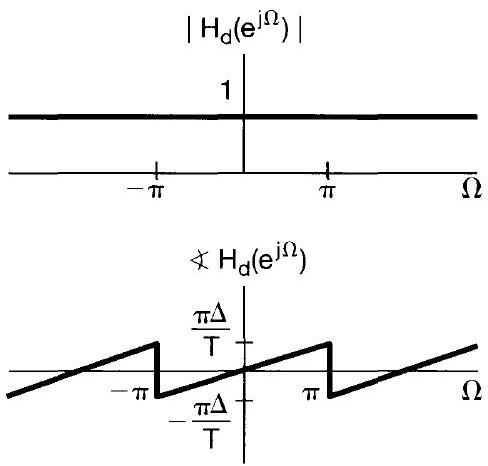
Corresponding \(H_d(e^{j\Omega})\)
Discrete-Time Decimation (Downsampling)
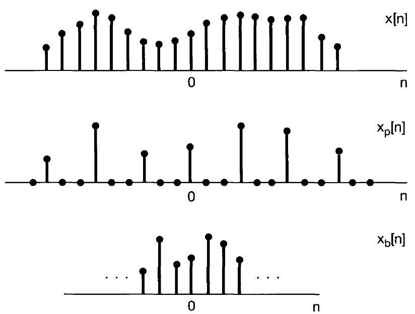
Sampling vs. Decimation
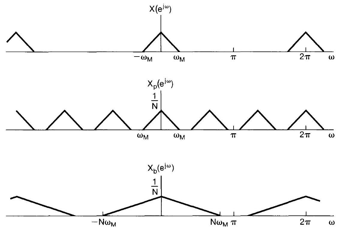
Effect of decimation in frequency domain
Example: Combined Decimation and Interpolation
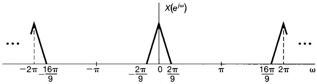
Original \(X(e^{j\omega})\)
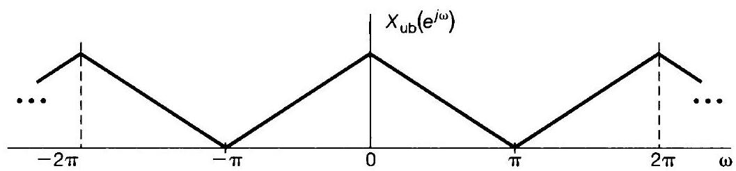
Final spectrum after rate change by 2/9
Note
This technique is vital in multi-rate signal processing, allowing efficient conversion between different sampling rates.