Signals and Systems

7.2 Signal Reconstruction

Imron Rosyadi

Signal Reconstruction

From Samples to Continuous Signals

Good morning everyone! Today, we’re diving into a crucial topic in Signals and Systems: how we reconstruct a continuous signal from its discrete samples. This is fundamental for digital signal processing, communication, and many other ECE applications. We’ll explore both theoretical ideal reconstruction and practical, real-world methods.

The Challenge of Reconstruction

• Digital World: Most modern systems process signals in discrete, sampled form.
• Analog World: Our physical world, however, is inherently continuous.
• The Bridge: How do we convert back from discrete samples to a continuous signal that accurately represents the original?

Important

Goal: To recover the original continuous-time signal \(x(t)\) from its discrete samples \(x(nT)\).

Figure 7.9: Linear interpolation between sample points. The dashed curve represents the original signal and the solid curve the linear interpolation.

Think about your smartphone or a digital music player. Sounds are continuous waves, but they are sampled and stored digitally. When you play music, your device needs to reconstruct that continuous sound wave from the digital samples. This slide sets up the core problem we’re addressing. We’re essentially trying to “fill in the gaps” between the discrete samples to get a smooth, continuous signal. The image here gives a preview of one simple way to do that: linear interpolation, where we connect the dots with straight lines.

Ideal Reconstruction: The Sampling Theorem’s Promise

• Recall: For a band-limited signal \(x(t)\) with maximum frequency \(\omega_M\), if sampled at a rate \(\omega_s \ge 2\omega_M\) (Nyquist rate), exact reconstruction is theoretically possible.
• The Tool: An ideal lowpass filter.

System Model:

• Samples \(x(nT)\) are converted to an impulse train \(x_p(t)\).
• This impulse train passes through an ideal lowpass filter \(H(j\omega)\).
• The output \(x_r(t)\) is the reconstructed signal.

\[ x_{r}(t)=x_{p}(t) * h(t) \] Where \(h(t)\) is the impulse response of the ideal lowpass filter.

Before we dive into practical interpolation methods, it’s crucial to remember the theoretical foundation: the Sampling Theorem. It tells us when exact reconstruction is possible. If we sample fast enough, we haven’t lost any information. The key to this ideal reconstruction is using an ideal lowpass filter. This filter essentially “smooths out” the impulse train, recovering the original continuous signal. The diagram illustrates this conceptual process, showing the signal flow from analog to sampled impulses, then through the filter to the reconstructed signal.

The Ideal Interpolation Formula

• The impulse response of an ideal lowpass filter is the sinc function. \[ h(t)=\frac{\omega_{c} T \sin \left(\omega_{c} t\right)}{\pi \omega_{c} t} \quad \text{where } \omega_c = \omega_s / 2 \]
• Substituting \(h(t)\) into the convolution equation:

\[ x_{r}(t)=\sum_{n=-\infty}^{+\infty} x(n T) \frac{\omega_{c} T}{\pi} \frac{\sin \left(\omega_{c}(t-n T)\right)}{\omega_{c}(t-n T)} \tag{7.11} \]

Note

This equation describes band-limited interpolation. It shows that the reconstructed signal is a superposition of scaled and shifted sinc functions, where each sample \(x(nT)\) determines the amplitude of a sinc function centered at \(nT\).

This is the mathematical core of ideal reconstruction. The impulse response of an ideal lowpass filter is not just any function; it’s the famous sinc function. When we convolve our sampled impulse train with this sinc function, the result is this infinite summation. Each sample point \(x(nT)\) acts as a weight for a sinc function that is shifted to that specific sample instant. The sinc function has a crucial property: it’s zero at all integer multiples of its period except at its center. This makes it perfect for interpolation, as each sinc function contributes only at its own sample point and is zero at the locations of other sample points.

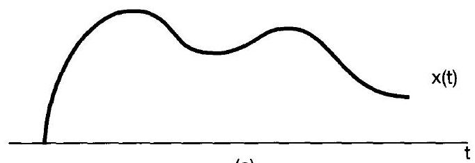
Visualizing Ideal Band-Limited Interpolation

• Original Signal \(x(t)\): A smooth, band-limited signal.
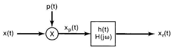
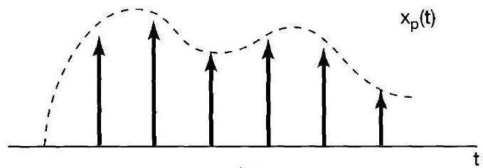
• Impulse Train \(x_p(t)\): The signal represented by discrete impulses at sampling instants.
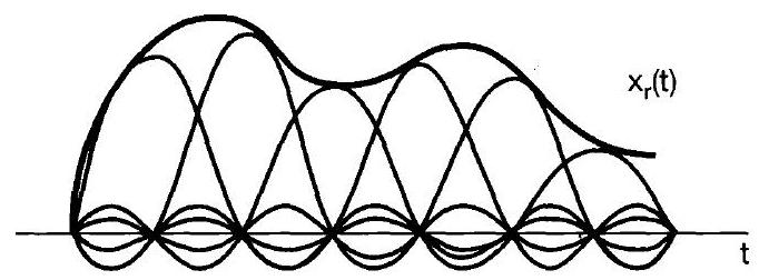
• Superposition of Sincs: Each impulse is effectively replaced by a scaled sinc function. Their sum perfectly reconstructs \(x(t)\).

(a) Band-limited signal \(x(t)\)

(b) Impulse train of samples of \(x(t)\)

(c) Ideal band-limited interpolation

These figures beautifully illustrate the concept of ideal reconstruction. Figure (a) is our original continuous signal. Figure (b) shows the discrete samples represented as impulses at the sampling instants. Then, in Figure (c), you see how each impulse is “spread out” into a sinc function. When all these scaled and shifted sinc functions are added together, they perfectly sum up to the original continuous signal. This is the magic of the sampling theorem and ideal lowpass filtering in action.

The Sinc Function: The Ideal Interpolator

• The sinc function (normalized form sin(πx)/(πx)) is crucial for ideal reconstruction.
• It’s an oscillatory function that decays over time.
• Its Fourier Transform is a rectangular pulse (the ideal lowpass filter frequency response).

Tip

Key Property:

sinc(0) = 1

sinc(n) = 0 for all non-zero integers n.

This ensures that at each sample point nT, only \(x(nT)\) contributes, and at other sample points kT (where k != n), \(x(nT)\)’s sinc function is zero.

The Sinc Function: The Ideal Interpolator

Interactive Sinc Function

viewof sinc_amp = Inputs.range([0.5, 2.0], {value: 1, step: 0.1, label: "Amplitude"});
viewof sinc_freq = Inputs.range([0.1, 5.0], {value: 1, step: 0.1, label: "Frequency Scale"});

The sinc function is truly remarkable. Its unique property of being zero at all non-zero integer multiples makes it the perfect building block for ideal interpolation. When you adjust the frequency scale using the slider, you can see how the width of the main lobe changes, which corresponds to the cutoff frequency of the ideal lowpass filter. A wider sinc in the time domain implies a narrower bandwidth in the frequency domain, and vice-versa. This interactive plot helps visualize these key characteristics.

Practical Interpolation: Zero-Order Hold (ZOH)

• Ideal filters are non-causal and unrealizable.
• We need simpler, practical interpolators.
• Zero-Order Hold (ZOH): The simplest form of interpolation.
  • Holds the value of each sample until the next sample arrives.
  • Produces a “stair-step” or “mosaic” effect.

Impulse Response (\(h_0(t)\)):

• A rectangular pulse of duration \(T\) (sampling period).
  • \(h_0(t) = 1\) for \(0 \le t < T\)
  • \(h_0(t) = 0\) otherwise

Output: - \(x_0(t) = \sum_{n=-\infty}^{+\infty} x(nT) h_0(t-nT)\)

Warning

Limitation: A very rough approximation. The output is discontinuous.

While ideal reconstruction is theoretically perfect, it’s not physically implementable because ideal lowpass filters are non-causal. So, in practice, we use approximations. The simplest is the Zero-Order Hold. It’s like taking a snapshot of a signal’s value and holding that value constant until the next snapshot arrives. This creates a blocky, stair-step signal. The image here clearly shows the “mosaic effect” this creates in 2D signals like images. Despite its roughness, it’s widely used in many digital-to-analog converters (DACs) due to its simplicity.

ZOH Transfer Function & Limitations

• The ZOH can be viewed as an approximation to the ideal lowpass filter.
• Its transfer function is not ideal.

\[ H_0(j\omega) = T \frac{\sin(\omega T/2)}{\omega T/2} e^{-j\omega T/2} \] The magnitude, \(|H_0(j\omega)|\), has a sinc function (unnormalized) shape.

• Pros: Simple, easy to implement in hardware.
• Cons:
  • Significant high-frequency content (not a perfect lowpass filter).
  • Introduces distortion and aliasing artifacts if not followed by a good analog lowpass filter.
  • Output is discontinuous.

Here we compare the ZOH’s frequency response to the ideal one. Notice how the ZOH’s magnitude response is not a perfect rectangle; it rolls off gradually and has side lobes. This means it doesn’t perfectly block high frequencies and can introduce some spectral distortion. This non-ideal behavior is why the ZOH produces a “rough” reconstruction. However, as the text notes, sometimes it’s “sufficient,” especially if further lowpass filtering is applied by the system or even by the human visual system, as seen in the image example from the previous slide.

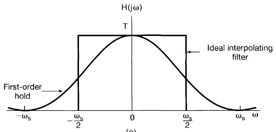
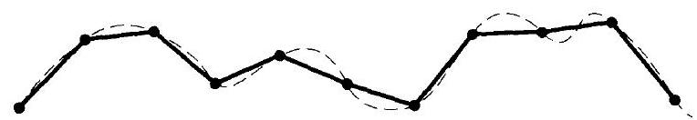
Practical Interpolation: First-Order Hold (Linear Interpolation)

• First-Order Hold (FOH): Connects adjacent sample points with a straight line.
• Provides a smoother output than ZOH.
• Also known as linear interpolation.

Impulse Response (\(h_1(t)\)):

• A triangular pulse of duration \(2T\), centered at \(T\).
  • \(h_1(t)\) increases linearly from 0 to 1 for \(0 \le t \le T\).
  • \(h_1(t)\) decreases linearly from 1 to 0 for \(T < t \le 2T\).
  • \(h_1(t) = 0\) otherwise.

Output: - Continuous, but with discontinuous derivatives (sharp corners at sample points).

Tip

Improvement: FOH offers a better approximation to the ideal filter compared to ZOH.

(a) System for sampling and reconstruction (with FOH impulse response)

(e) Comparison of transfer function of ideal interpolating filter (solid) and first-order hold (dashed).

Moving up in complexity, the First-Order Hold, or linear interpolation, is a significant improvement over ZOH. Instead of holding the value, it draws a straight line between consecutive samples. This gives us a continuous output, which is generally more desirable. The image illustrates the system model and, more importantly, compares its frequency response to the ideal one. You can see it’s a better fit than the ZOH, especially near DC, meaning it performs better as a lowpass filter.

FOH Transfer Function & Higher-Order Holds

• The FOH also has a non-ideal transfer function, but it’s closer to ideal than ZOH.

\[ H(j \omega)=\frac{1}{T}\left[\frac{\sin (\omega T / 2)}{\omega / 2}\right]^{2} \tag{7.12} \]

• This is essentially the square of the ZOH magnitude response (with some scaling).

Important

Higher-Order Holds:

• Can use higher-order polynomials for interpolation (e.g., cubic splines).
• Provide even smoother reconstructions with continuous derivatives.
• Come with increased computational complexity and potential for overshoot.

The transfer function of the FOH has a sinc^2 shape, which generally provides a better lowpass characteristic than the sinc shape of the ZOH. This means it attenuates high frequencies more effectively, leading to a smoother output. While FOH is good, we can go even further with higher-order holds. These use more complex polynomial functions to fit the samples, resulting in even smoother outputs, potentially with continuous first or second derivatives. However, there’s always a trade-off between reconstruction quality, computational cost, and potential artifacts like overshoot or ringing.

Interactive Interpolation Comparison

• Observe the effects of ZOH and FOH on a sampled sine wave.
• Adjust the sampling rate to see how it impacts reconstruction quality.

viewof sampling_rate = Inputs.range([5, 50], {value: 10, step: 1, label: "Sampling Rate (samples/period)"});
viewof signal_freq = Inputs.range([0.5, 5.0], {value: 1, step: 0.1, label: "Signal Frequency (Hz)"});
viewof amplitude = Inputs.range([0.5, 2.0], {value: 1, step: 0.1, label: "Amplitude"});

This interactive plot allows you to directly compare the performance of ZOH and linear interpolation. Notice how the ZOH creates those sharp steps, while linear interpolation connects the dots with straight lines, making it smoother. Pay close attention to what happens when you decrease the sampling rate. The reconstructions become less accurate, highlighting the importance of the Nyquist sampling criterion, even for approximate methods. At very low sampling rates, both methods struggle to represent the original signal faithfully. Experiment with different signal frequencies and amplitudes as well.

Summary & Key Takeaways

• Reconstruction Goal: Convert discrete samples back to a continuous signal.
• Ideal Reconstruction: Achieved with an ideal lowpass filter (sinc function) if Nyquist criterion is met.
  • Theoretically perfect, but practically unrealizable (non-causal).
• Practical Interpolation:
  • Zero-Order Hold (ZOH): Simple, “stair-step” output, discontinuous.
  • First-Order Hold (FOH) / Linear Interpolation: Smoother, continuous output, but with discontinuous derivatives.
  • Higher-order holds offer greater smoothness at increased complexity.

Tip

Engineering Trade-offs:

Choosing an interpolation method involves balancing:

1. Accuracy: How close is the reconstructed signal to the original?
2. Complexity: Computational cost and hardware requirements (e.g., memory, processing power).
3. Real-time Constraints: Can it be done fast enough for the application?
4. Application Needs: What level of smoothness/fidelity is acceptable? (e.g., audio vs. control systems).

To wrap up, remember that signal reconstruction is a fundamental process in ECE. While ideal reconstruction gives us a theoretical benchmark, practical systems rely on approximations like ZOH and FOH. The choice of interpolator is a classic engineering trade-off. We always balance the desired accuracy with the available resources and the specific requirements of the application. For instance, a simple audio playback might use a higher-order hold for better fidelity, while a control system might use a ZOH for simplicity and speed, especially for digital-to-analog conversion before an actuator.