Signals and Systems

7.1 The Sampling Theorem

Imron Rosyadi

The Sampling Theorem: Bridging Continuous and Discrete Signals

Introduction to Sampling: The Digital Frontier

Signals in the real world are often continuous-time (analog). However, modern systems (computers, digital communication) operate on discrete-time (digital) signals.

Sampling is the process of converting a continuous-time signal into a discrete-time sequence.

• Why Sample?
  • Digital processing advantages (noise immunity, flexibility).
  • Storage and transmission efficiency.
  • Enables powerful digital signal processing (DSP) algorithms.

Figure 7.1: Three continuous-time signals with identical values at integer multiples of \(T\).

Note

Key Question: How do we convert an analog signal to digital without losing information?

Good morning, everyone! Today we’re diving into a fundamental concept in Signals and Systems: the Sampling Theorem. This theorem is the bridge between the analog world we live in and the digital world our computers and smartphones operate in. We’ll explore why sampling is necessary, how it works, and what conditions are required to ensure we don’t lose crucial information during this conversion. As you can see in Figure 7.1, simply taking samples isn’t enough; many different continuous signals can produce the same set of discrete samples. Our goal is to understand how to make this conversion unique and reversible.

The Challenge: Ambiguity in Sampling

From Figure 7.1, it’s clear:

• An infinite number of continuous-time signals can pass through the same discrete samples.
• Without additional information, samples alone don’t uniquely define the original signal.

Our Goal: Find conditions under which a signal can be uniquely specified by its samples, allowing perfect reconstruction.

Important

This unique specification is possible if the signal is band-limited and sampled at a sufficiently high rate.

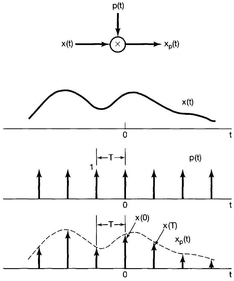
Impulse-Train Sampling: The Model

To analyze sampling mathematically, we use impulse-train sampling.

1. Continuous Signal: \(x(t)\)
2. Sampling Function: A periodic impulse train \(p(t)\). \[ p(t)=\sum_{n=-\infty}^{+\infty} \delta(t-n T) \]
   • \(T\): Sampling Period
   • \(\omega_s = 2\pi/T\): Sampling Frequency
3. Sampled Signal: \(x_p(t) = x(t)p(t)\)

Using the sampling property of the impulse: \[ x_p(t)=\sum_{n=-\infty}^{+\infty} x(n T) \delta(t-n T) \] This produces an impulse train where each impulse’s amplitude is the value of \(x(t)\) at the sampling instant \(nT\).

Figure 7.2: Impulse-train sampling.

Impulse-train sampling is a theoretical model that simplifies the analysis of sampling. We multiply our continuous signal \(x(t)\) by a train of impulses. Each impulse is like a tiny “snapshot” of the signal’s value at that specific time instant. The resulting signal, \(x_p(t)\), is a series of weighted impulses, where the weights are precisely the samples of the original signal. This representation is crucial because it allows us to analyze the sampling process in the frequency domain using the Fourier Transform.

Sampling in the Frequency Domain: Replicas

The magic happens in the frequency domain.

• Multiplication in the time domain corresponds to convolution in the frequency domain. \[ X_p(j\omega) = \frac{1}{2\pi} [X(j\omega) * P(j\omega)] \]
• The Fourier Transform of the impulse train \(p(t)\) is also an impulse train in frequency: \[ P(j\omega) = \frac{2\pi}{T} \sum_{k=-\infty}^{+\infty} \delta(\omega - k\omega_s) \]
• Convolving \(X(j\omega)\) with \(P(j\omega)\) gives: \[ X_p(j\omega) = \frac{1}{T} \sum_{k=-\infty}^{+\infty} X(j(\omega - k\omega_s)) \]

Tip

Interpretation: The spectrum of the sampled signal, \(X_p(j\omega)\), is an infinite sum of shifted and scaled replicas of the original signal’s spectrum, \(X(j\omega)\). Each replica is centered at multiples of the sampling frequency \(\omega_s\).

When we move to the frequency domain, the multiplication of \(x(t)\) and \(p(t)\) becomes a convolution of their Fourier Transforms. Since \(p(t)\) is an impulse train, its Fourier Transform \(P(j\omega)\) is also an impulse train, but in the frequency domain. The convolution operation then effectively creates multiple copies of the original signal’s spectrum, \(X(j\omega)\), shifted by integer multiples of the sampling frequency, \(\omega_s\). These are called spectral replicas. The key insight here is how these replicas interact.

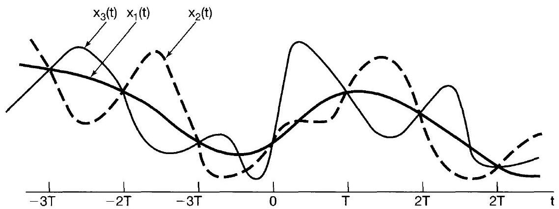
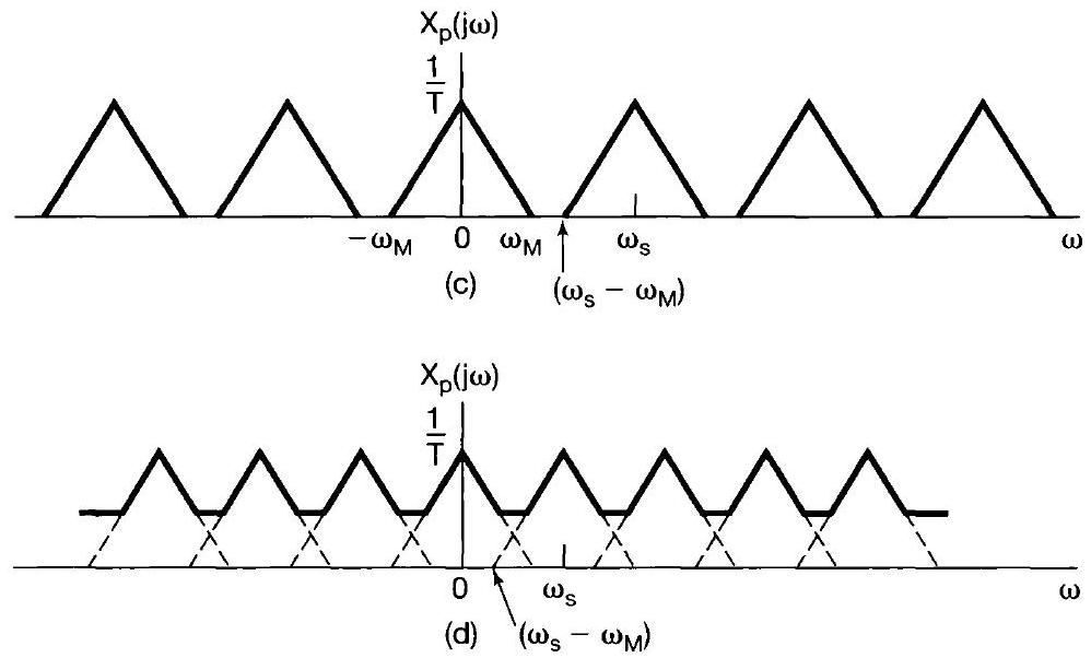
Aliasing: When Replicas Overlap

The relationship between the sampling frequency (\(\omega_s\)) and the signal’s bandwidth (\(\omega_M\)) is critical.

Case 1: No Overlap (\(\omega_s > 2\omega_M\))

• The replicas of \(X(j\omega)\) are perfectly separated.
• The original spectrum \(X(j\omega)\) can be recovered by an ideal lowpass filter.

Case 2: Overlap (\(\omega_s < 2\omega_M\))

• The replicas overlap, causing aliasing.
• Information is lost; the original signal cannot be perfectly reconstructed.

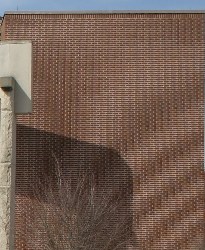
Figure 7.3 (c) and (d): Spectrum of sampled signal with \(\omega_{s}>2 \omega_{M}\) (no aliasing) and \(\omega_{s}<2 \omega_{M}\) (aliasing).

This is where the concept of aliasing comes into play. If our sampling frequency \(\omega_s\) is high enough, specifically greater than twice the highest frequency component in our original signal, \(\omega_M\), then the spectral replicas are well-separated. We can then use a simple lowpass filter to isolate the original spectrum and perfectly reconstruct the signal. However, if \(\omega_s\) is too low, the replicas overlap. This overlap is called aliasing, and it causes higher frequencies in the original signal to appear as lower frequencies in the sampled signal, leading to irreversible distortion.

Interactive: Exploring Aliasing

Adjust the signal bandwidth (\(\omega_M\)) and sampling frequency (\(\omega_s\)) to observe aliasing.

viewof signal_bandwidth = Inputs.range([0.1, 5.0], {value: 1.0, step: 0.1, label: "Signal Bandwidth (ω_M)"});
viewof sampling_frequency = Inputs.range([0.1, 10.0], {value: 3.0, step: 0.1, label: "Sampling Frequency (ω_s)"});

This interactive plot helps visualize the core concept of aliasing. The blue line represents the Fourier Transform of our original band-limited signal. The red dashed line shows the spectrum after impulse-train sampling. As you adjust the “Signal Bandwidth” (\(\omega_M\)) and “Sampling Frequency” (\(\omega_s\)), you can see how the replicas of the original spectrum shift and potentially overlap. Pay close attention to when the “Aliasing Occurring!” message appears – this is when \(\omega_s\) drops below the Nyquist rate, \(2\omega_M\), and reconstruction becomes impossible.

Aliasing in Images

Motorcycle: low resolution, Moire

Motorcycle: high resolution

Brick: low resolution, Moire

Brick: high resolution

Aliasing in Videos

The Sampling Theorem

Formal Statement:

Let \(x(t)\) be a band-limited signal with \(X(j\omega)=0\) for \(|\omega| > \omega_M\). Then \(x(t)\) is uniquely determined by its samples \(x(nT), n=0, \pm 1, \pm 2, \ldots\), if

\[ \omega_s > 2\omega_M \]

where \(\omega_s = 2\pi/T\) is the sampling frequency.

Note

The frequency \(2\omega_M\) is known as the Nyquist rate. \(\omega_M\) is often called the Nyquist frequency.

The Sampling Theorem

Reconstruction Process

1. Generate an impulse train \(x_p(t)\) from the samples.
2. Pass \(x_p(t)\) through an ideal lowpass filter with:
   • Gain \(T\)
   • Cutoff frequency \(\omega_c\) such that \(\omega_M < \omega_c < \omega_s - \omega_M\).

The output signal will exactly equal \(x(t)\).

This is the formal statement of the Sampling Theorem. It provides the crucial condition for perfect reconstruction: the sampling frequency must be strictly greater than twice the highest frequency component in the signal. The term \(2\omega_M\) is so important that it has its own name: the Nyquist rate. To reconstruct the signal, we essentially reverse the sampling process in the frequency domain. We take our sampled impulse train, whose spectrum contains the original spectrum and its replicas, and pass it through an ideal lowpass filter. This filter acts like a “sieve,” isolating just the original baseband spectrum and filtering out all the higher-frequency replicas. The gain \(T\) is necessary to restore the original amplitude scaling.

Ideal Reconstruction: The Lowpass Filter

The ideal lowpass filter \(H(j\omega)\) has: \[ H(j\omega) = \begin{cases} T & |\omega| < \omega_c \\ 0 & |\omega| \ge \omega_c \end{cases} \] where \(\omega_M < \omega_c < \omega_s - \omega_M\).

This filter effectively isolates the baseband spectrum \(X(j\omega)\) from its replicas, scaled by \(T\) to restore the original amplitude.

Figure 7.4 (a) and (d): System for sampling and reconstruction, and the ideal lowpass filter.

Figure 7.4 illustrates the complete system for sampling and reconstruction. The sampled signal \(x_p(t)\) goes through an ideal lowpass filter. This filter’s job is to perfectly cut off all the spectral replicas, leaving only the original signal’s spectrum in its passband. The gain of \(T\) is applied to counteract the \(1/T\) scaling introduced during sampling, ensuring the reconstructed signal has the correct amplitude. While ideal filters are not physically realizable, they provide a theoretical benchmark and are approximated by practical filters in real-world applications.

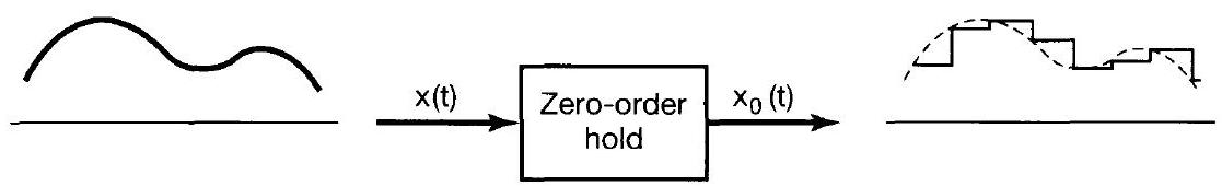
Practical Sampling: Zero-Order Hold

Impulse-train sampling is theoretical. In practice, a zero-order hold is often used.

• Samples \(x(t)\) at an instant and holds that value until the next sample.
• Output \(x_0(t)\) is a staircase-like approximation of \(x(t)\).

Figure 7.5: Sampling utilizing a zero-order hold.

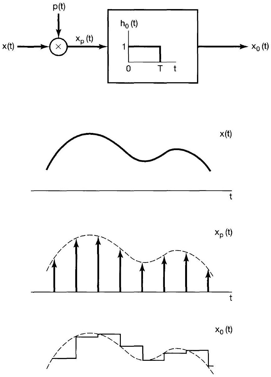
Representation: A zero-order hold can be modeled as impulse-train sampling followed by an LTI system with a rectangular impulse response \(h_0(t)\): \[ h_0(t) = \begin{cases} 1 & 0 \le t < T \\ 0 & \text{otherwise} \end{cases} \]

Figure 7.6: Zero-order hold as impulse-train sampling followed by an LTI system with a rectangular impulse response.

While impulse-train sampling is great for theoretical analysis, it’s not what physically happens in most Analog-to-Digital Converters (ADCs). A more practical approach is the zero-order hold. Imagine a sample-and-hold circuit: it takes a sample and then holds that voltage level constant until the next sample arrives. This creates a staircase-like approximation of the original signal. We can model this by first performing impulse-train sampling and then passing the resulting impulses through a system with a rectangular impulse response, essentially “stretching” each impulse into a pulse of duration \(T\).

Zero-Order Hold: Reconstruction

To reconstruct \(x(t)\) from \(x_0(t)\), we need a specific filter.

The Fourier Transform of \(h_0(t)\) is: \[ H_0(j\omega) = e^{-j\omega T/2} \left[ \frac{2\sin(\omega T/2)}{\omega} \right] \] This is a sinc function in frequency.

To reconstruct \(x(t)\), we need to compensate for \(H_0(j\omega)\).

The reconstruction filter \(H_r(j\omega)\) must satisfy: \[ H_r(j\omega) H_0(j\omega) = H_{ideal}(j\omega) \] Where \(H_{ideal}(j\omega)\) is the ideal lowpass filter with gain \(T\).

Thus, the required reconstruction filter is: \[ H_r(j\omega) = \frac{e^{j\omega T/2} H_{ideal}(j\omega)}{\frac{2\sin(\omega T/2)}{\omega}} \]

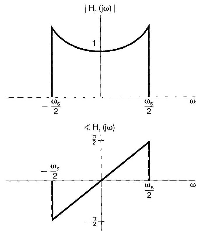
Figure 7.8: Magnitude and phase for the reconstruction filter for a zero-order hold.

Caution

This reconstruction filter is complex to implement due to the sinc inverse in the denominator and the non-constant gain in the passband.

Since the zero-order hold introduces its own frequency response, \(H_0(j\omega)\), during the sampling process, our reconstruction filter needs to undo that effect in addition to performing the lowpass filtering. This means the reconstruction filter \(H_r(j\omega)\) will have a more complex characteristic than a simple ideal lowpass filter. As shown in Figure 7.8, its magnitude is not flat, and its phase is not linear, making it more challenging to implement in practice compared to the ideal lowpass filter for impulse-train sampling. Often, in many applications, the output of the zero-order hold itself is considered a sufficient approximation, or more sophisticated interpolation methods are used.

Interactive: Zero-Order Hold in Time Domain

Observe how a continuous signal is approximated by a zero-order hold for different sampling periods.

viewof signal_freq = Inputs.range([0.1, 2.0], {value: 0.5, step: 0.1, label: "Signal Frequency (Hz)"});
viewof sampling_period = Inputs.range([0.05, 1.0], {value: 0.2, step: 0.01, label: "Sampling Period (T)"});

This interactive plot demonstrates the zero-order hold in the time domain. The blue curve is our original continuous-time signal, a simple sine wave. The red markers are the discrete samples taken at intervals of \(T\). The green dotted line shows the output of the zero-order hold. As you decrease the “Sampling Period (T)”, which means increasing the sampling frequency, you’ll notice that the staircase-like approximation of the zero-order hold becomes much smoother and more closely resembles the original signal. This visually reinforces the idea that a higher sampling rate generally leads to a better approximation and easier reconstruction.

Conclusion & Applications

Key Takeaways:

• Sampling Theory provides the mathematical foundation for converting analog to digital signals.
• The Sampling Theorem states that a band-limited signal can be perfectly reconstructed from its samples if the sampling frequency \(\omega_s\) is greater than the Nyquist rate (\(2\omega_M\)).
• Aliasing occurs when the sampling rate is too low, leading to irreversible loss of information.
• Zero-Order Hold is a practical method for sampling, requiring a more complex reconstruction filter.

Conclusion & Applications

Real-World ECE Applications:

• Analog-to-Digital Converters (ADCs): Crucial components in almost all digital systems (audio, video, sensors).
• Digital Audio: CDs (44.1 kHz sampling rate) and high-resolution audio.
• Digital Image Processing: Pixels are samples of continuous light intensity.
• Telecommunications: Digital modulation and demodulation.
• Control Systems: Sampling sensor data for feedback.

Tip

Understanding the Sampling Theorem is fundamental for designing robust and accurate digital signal processing systems.

In summary, the Sampling Theorem is a cornerstone of modern ECE. It tells us not just that we can convert analog signals to digital, but how to do it correctly to avoid losing information. From the music you listen to, to the images on your screen, to the complex control systems in modern machinery, the principles of sampling are at play everywhere. Ignoring the Nyquist rate can lead to significant problems, such as distorted audio or inaccurate sensor readings. So, while the math can seem abstract, its practical implications are vast and critical to virtually every aspect of electrical and computer engineering.