Signal and Systems

1.5 Continuous-Time and Discrete-Time Systems

Imron Rosyadi

1.5 Continuous-Time and Discrete-Time Systems

What is a System?

A system is a process by which input signals are transformed to produce output signals.

Conceptual Model:

graph LR
    A[Input Signal] --> B(System);
    B --> C[Output Signal];

Examples:

• Hi-Fi System: Raw audio \(\rightarrow\) Amplified & Equalized sound
• RC Circuit: Input voltage \(\rightarrow\) Capacitor voltage
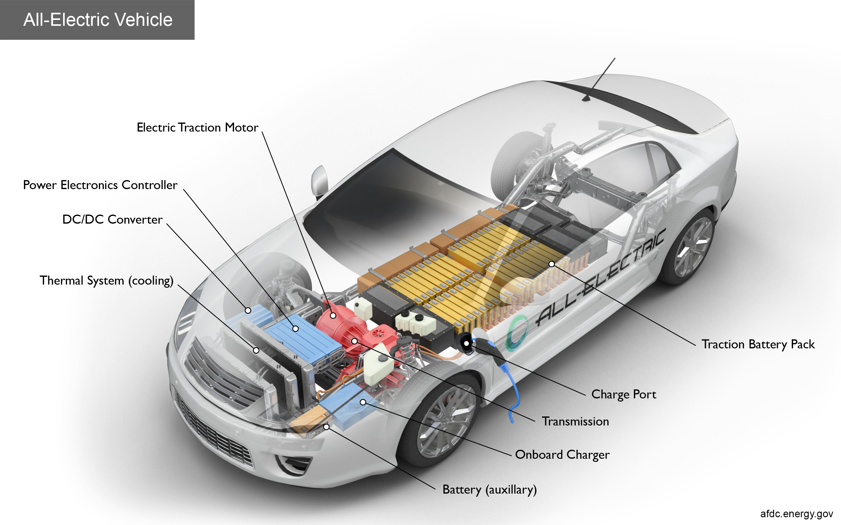
• Automobile: Force applied \(\rightarrow\) Vehicle velocity
• Image Enhancement: Raw image \(\rightarrow\) Improved contrast image

Key Idea:

Systems provide a mathematical framework to model how physical phenomena respond to external stimuli.

They allow us to predict, control, and design complex engineering applications.

In the broadest sense, a system is simply anything that takes an input and produces an output. Think of it as a black box where something goes in, is processed, and something else comes out. In electrical and computer engineering, these inputs and outputs are typically signals, and the “processing” is defined by mathematical relationships. We analyze these relationships to understand how a system behaves.

Systems (Examples)

Systems (Examples)

Continuous-Time (CT) vs. Discrete-Time (DT) Systems

Systems are classified based on the nature of their input and output signals.

Continuous-Time Systems

• Input \(x(t)\) and output \(y(t)\) are continuous functions of time.
• Represented by: \(x(t) \rightarrow y(t)\)

Real-world examples:

• Analog filters
• Mechanical systems
• Electrical circuits (e.g., op-amp circuits)

Discrete-Time Systems

• Input \(x[n]\) and output \(y[n]\) are sequences (defined at discrete instants).
• Represented by: \(x[n] \rightarrow y[n]\)

Real-world examples:

• Digital signal processors (DSPs)
• Computer algorithms
• Financial modeling (e.g., monthly balances)

The fundamental distinction lies in how time is handled. Continuous-time systems operate on signals that are defined for all values of time, much like a continuous waveform. Discrete-time systems, on the other hand, operate on signals that are sampled or defined only at specific, discrete points in time. We will study both types in parallel throughout this course, but in Chapter 7, we’ll see how they are connected through the concept of sampling. Many real-world systems, especially in modern engineering, involve both, for example, processing an analog signal using a digital computer.

Simple Examples of Systems: Continuous-Time (1/2)

Many diverse physical systems can share the same mathematical description.

Example 1.8: RC Circuit Voltage

System: An RC circuit where \(v_s(t)\) is the input voltage and \(v_c(t)\) is the output voltage across the capacitor.

Input-Output Relationship (Differential Equation): \[ \frac{d v_{c}(t)}{d t}+\frac{1}{R C} v_{c}(t)=\frac{1}{R C} v_{s}(t) \quad \text{(Equation 1.82)} \]

Let’s look at some basic examples. Consider a simple RC circuit. The input is the source voltage vs(t) and the output is the capacitor voltage vc(t). Using Kirchhoff’s laws and the constitutive relations for resistors and capacitors, we can derive a first-order differential equation that describes how the output voltage vc(t) changes in response to the input voltage vs(t). This equation captures the dynamics of the circuit.

Simple Examples of Systems: Continuous-Time (2/2)

Example 1.9: Automobile Velocity

System: An automobile where \(f(t)\) is the input force and \(v(t)\) is the output velocity. (Assumes mass \(m\) and friction \(\rho v\)).

Input-Output Relationship (Differential Equation): \[ \frac{d v(t)}{d t}+\frac{\rho}{m} v(t)=\frac{1}{m} f(t) \quad \text{(Equation 1.84)} \]

Simple Examples of Systems: Continuous-Time (2/2)

Comparison: Both Example 1.8 (RC circuit) and 1.9 (automobile) are described by the same general first-order linear differential equation:

\[ \frac{d y(t)}{d t}+a y(t)=b x(t) \quad \text{(Equation 1.85)} \]

• \(y(t)\): output signal, \(x(t)\): input signal.
• \(a\), \(b\): constants derived from system parameters.

Now, let’s consider a completely different physical system: an automobile. If we model the applied force f(t) as the input and the vehicle’s velocity v(t) as the output, and account for mass and a linear approximation for frictional resistance, Newton’s second law leads us to another first-order differential equation.

What’s striking is that this equation has the exact same mathematical form as the RC circuit equation. This demonstrates a powerful concept in systems analysis: seemingly different physical systems can be described by the same mathematical models. Developing tools to analyze a general class of systems, like first-order linear differential equations, allows us to apply those tools across a wide variety of engineering disciplines.

Simple Examples of Systems: Discrete-Time (1/2)

Example 1.10: Bank Account Balance

System: A bank account where \(x[n]\) is the net deposit in month \(n\), and \(y[n]\) is the balance at the end of month \(n\). (Assumes 1% interest per month).

Input-Output Relationship (Difference Equation): \[ y[n] = 1.01 y[n-1] + x[n] \quad \text{(Equation 1.86)} \] \[ y[n] - 1.01 y[n-1] = x[n] \quad \text{(Equation 1.87)} \]

Simple Examples of Systems: Discrete-Time (1/2)

Example 1.10: Bank Account Balance

Interactive Simulation: Assume initial balance \(y[-1]=1000\) and a monthly deposit \(x[n]=100\) for \(n \ge 0\). The system calculates balance \(y[n]\) based on previous month’s balance and current deposit.

Discrete-time systems are modeled using difference equations. A classic example is tracking a bank account balance. Here, the current month’s balance, y[n], depends on the previous month’s balance, y[n-1], augmented by interest, and the current month’s net deposit, x[n]. This difference equation captures the temporal evolution of the balance. The interactive plot shows how the balance grows over time with regular deposits and compounding interest.

Simple Examples of Systems: Discrete-Time (2/2)

Example 1.11: Digital Simulation of Automobile Model

System: A discrete-time approximation of the continuous-time automobile model from Example 1.9. (Approximates \(\frac{dv(t)}{dt}\) with backward difference \(\frac{v(n\Delta)-v((n-1)\Delta)}{\Delta}\)).

Input-Output Relationship (Difference Equation): \[ v[n]-\frac{m}{(m+\rho \Delta)} v[n-1]=\frac{\Delta}{(m+\rho \Delta)} f[n] \quad \text{(Equation 1.88)} \]

• \(v[n]\): sampled velocity, \(f[n]\): sampled force.
• \(\Delta\): time step.

Simple Examples of Systems: Discrete-Time (2/2)

Comparison: Both Example 1.10 (bank account) and 1.11 (digital simulation) are described by the same general first-order linear difference equation:

\[ y[n]+a y[n-1]=b x[n] \quad \text{(Equation 1.89)} \]

• \(y[n]\): output sequence, \(x[n]\): input sequence.
• \(a\), \(b\): constants derived from system parameters or approximation schemes.

Just as with continuous-time systems, discrete-time systems from different applications can share the same mathematical form. Here, we see a digital simulation of the automobile model, where the continuous-time derivative is approximated by a discrete-time difference. This gives us a first-order linear difference equation. Comparing it to the bank account example, they both fit the same general form. This highlights the power of abstraction in signals and systems: by understanding general forms of equations, we can analyze countless real-world systems, whether they are inherently discrete or are continuous systems approximated for digital processing.

1.5.2 Interconnections of Systems

Complex systems are often built by interconnecting simpler subsystems.

• Benefit: Analyze complex systems by understanding their components and their connections.
• Application: Design and synthesize new systems from basic building blocks.

1.5.2 Interconnections of Systems

Real-World Application: Audio System

graph TD
    A[Radio Receiver] --> B(Amplifier);
    B --> C[Speakers];

An audio system cascaded for playback.

Real-World Application: Digitally Controlled Aircraft

graph TD
    Pilot[Pilot Commands] --> Autopilot(Digital Autopilot);
    Sensors --> Autopilot;
    Autopilot --> Actuators(Aircraft Actuators);
    Actuators --> Aircraft(Aircraft);
    Aircraft --> Sensors["Sensors (Velocity)"];
    Aircraft --> PilotsDisplay(Pilot Display);
    Autopilot --Desired--> Aircraft;
    Aircraft --Actual--> Autopilot;

    style Autopilot fill:#f9f
    style Aircraft fill:#cf9
    style Sensors fill:#9fc
    style Actuators fill:#c9f

A feedback system structure.

Most real-world engineering systems aren’t just one simple block. They are complex structures made by connecting several simpler components. Understanding how systems are interconnected is crucial for both analysis and design. By breaking down a large system into its component parts, we can apply our knowledge of the simpler subsystems and understand the overall behavior. This modular approach is fundamental in system engineering.

Basic Interconnections: Series (Cascade)

In a series or cascade interconnection, the output of one system becomes the input to the next.

graph LR
    input(Input) --> Sys1(System 1);
    Sys1 --> Sys2(System 2);
    Sys2 --> output(Output);

    subgraph Overall System
        Sys1
        Sys2
    end

• Description: Input signal is processed by System 1, then its output is processed by System 2.
• Example: A radio receiver (System 1) connected to an amplifier (System 2).
• Notation: If System 1 output = \(y_1\) and System 2 output = \(y_2\), then \(y_1 = \text{Sys1}(\text{input})\) and \(y_2 = \text{Sys2}(y_1)\).

The series or cascade interconnection is the most straightforward. Imagine a chain: the output of the first link feeds into the second, and so on. In block diagrams, this is represented by arrows connecting blocks sequentially. An example is a signal flowing from your phone to an amplifier, then to speakers. Each component performs a specific function in sequence.

Basic Interconnections: Parallel

In a parallel interconnection, the same input signal is applied to multiple systems, and their outputs are combined (typically summed).

graph LR
    input(Input) --> Sys1(System 1);
    input --> Sys2(System 2);
    Sys1 --> Sum;
    Sys2 --> Sum;
    Sum(($\oplus$)) --> output(Output);

    subgraph Overall System
        Sys1
        Sys2
        Sum
    end

• Description: Input simultaneously feeds System 1 and System 2. Their individual outputs are added together to form the overall output.
• Example: Multiple microphones (inputs) feeding into a mixing console (summing outputs) then to a single amplifier.

In a parallel interconnection, the input signal is duplicated and sent to two or more systems simultaneously. Their individual outputs are then combined, usually by addition, to form the final output. Think of it like a sound system with multiple microphones all feeding into a single mixer. Each microphone is a “system” producing an output, and the mixer sums these outputs.

Basic Interconnections: Feedback

In a feedback interconnection, the output of a system (or subsystem) is fed back and used to influence its own input.

graph LR
    input(External Input) --> Summer;
    System2_out(Output of S2) --> Summer;
    Summer(($\oplus$)) --> System1(System 1);
    System1 --> System2(System 2);
    System2 --> output(Output);
    System2_out -- Feedback --> Summer;

    subgraph Overall System
        Summer
        System1
        System2
    end

• Description: The output of System 2 is added (or subtracted) from the external input, which then becomes the effective input to System 1.
• Examples:
  • Cruise Control: Senses vehicle speed, adjusts engine to maintain desired speed.
  • Thermostat: Senses room temperature, turns heating/cooling on/off to reach set temperature.
  • Operational Amplifiers: Many op-amp circuits use feedback for stability and gain control.

Feedback is arguably the most powerful and common type of system interconnection. In a feedback system, part of the output is “fed back” to the input, influencing the system’s future behavior. This creates a closed loop. A common household example is a thermostat. It senses the room temperature (output), compares it to the desired temperature (input), and then adjusts the heating or cooling (actuator) to correct any difference. Feedback systems are essential for control, stability, and achieving precise performance in dynamic environments.

Key Takeaways

System Definition

• Transforms input signals into output signals.
• Can be continuous-time (\(x(t) \rightarrow y(t)\)) or discrete-time (\(x[n] \rightarrow y[n]\)).

Mathematical Models

• Continuous-time systems often described by differential equations.
• Discrete-time systems often described by difference equations.
• Many diverse physical systems share the same mathematical forms (e.g., first-order linear differential/difference equations).

Key Takeaways

System Interconnections

• Complex systems can be understood and built from simpler subsystems.
• Series (Cascade): Output of one system feeds the input of another.
• Parallel: Same input to multiple systems; outputs are combined.
• Feedback: Output of a system/subsystem is routed back to influence its input, crucial for control and stability.

Understanding these concepts is foundational for further study in Signals and Systems.

To wrap up our discussion on systems: Remember that a system is a fundamental concept where an input signal is transformed into an output signal. We differentiate between continuous-time systems, described by differential equations, and discrete-time systems, described by difference equations. A crucial takeaway is that the mathematical description of a system is often consistent across very different physical phenomena, providing a powerful framework for analysis. Finally, understanding how systems are interconnected—through series, parallel, or feedback arrangements—is key to analyzing complex real-world engineering systems and designing sophisticated solutions. These foundational concepts will be built upon throughout the course as we delve deeper into system properties and analysis techniques.