MH1810 Math

Chapter 4a: Limits and Continuity

Imron Rosyadi

Chapter 4: Limits and Continuity

Understanding fundamental concepts in Calculus.

• This chapter introduces the intuitive and formal definitions of limits.
• It explores different types of limits: one-sided, infinite, and limits at infinity.
• We will discuss limit theorems, practical evaluation techniques, and the concept of continuity.
• Finally, we’ll cover key theorems like the Intermediate Value Theorem and Extreme Value Theorem.

Welcome to Chapter 4: Limits and Continuity. This chapter is foundational for understanding calculus. We’ll start with the intuitive idea of a limit, then move to its formal definition. We will cover various types of limits including one-sided, infinite, and limits at infinity. A significant portion will be dedicated to limit theorems and practical techniques for evaluating limits. Finally, we’ll introduce the concept of continuity and explore important theorems like the Intermediate Value Theorem and the Extreme Value Theorem, which are crucial for analyzing function behavior.

4.1 Limit of a Function at a Point

Intuitive Idea of a Limit

What happens to \(f(x)\) for values of \(x\) near 2, when \(f(x) = x^2\)?

1. Computational Approach

Let’s look at values of \(f(x)\) as \(x\) gets closer to 2.

x	x²	x	x²
2.1	4.41	1.9	3.61
2.01	4.0401	1.99	3.9601
2.001	4.004001	1.999	3.996001
2.0001	4.00040001	1.9999	3.99960001

As \(x\) approaches 2, \(f(x)\) approaches 4.

2. Graphical Approach

Graph of \(f(x) = x^2\)

Observe the points on the graph of \(y=f(x)\) as \(x\) approaches 2. The y-values on the graph get closer to 4.

We write this as: \[\lim_{x \to 2} (x^2) = 4\]

The intuitive idea of a limit is about what value a function approaches as its input approaches a certain value. We can explore this concept using two methods: computationally and graphically.

Computationally: We see that as ‘x’ gets closer and closer to 2, from both sides, ‘f(x)’ or ‘x-squared’ gets closer and closer to 4. We are not interested in what happens at x equals 2, but what happens near 2.

Graphically: If you trace the graph of ‘y = x-squared’, as you move your finger along the x-axis towards 2, from both the left and the right, your finger on the y-axis will approach 4. This reinforces the idea that the function’s output approaches 4.

This observation, both numerically and visually, leads us to write the limit notation: the limit of x-squared as x approaches 2 is 4.

Definition of a Limit at a Point

Suppose \(f\) is defined near \(x = a\) (but not necessarily at \(x=a\)).

We say that \(f(x)\) approaches the limit \(L\) as \(x\) tends to \(a\), if we can make \(f(x)\) arbitrarily close to \(L\) by choosing \(x\) sufficiently close to \(a\).

We express this by writing: \[\lim_{x \to a} f(x) = L\]

Note

Key Points:

• Existence and Uniqueness: If \(\lim_{x \to a} f(x)\) exists, it means there is a unique real number \(L\).
• Non-existence: If there is no finite real number \(L\), then \(\lim_{x \to a} f(x)\) does not exist.

The formal definition of a limit at a point ‘a’ means that we can get the function’s output, ‘f(x)’, as close as we want to some value ‘L’, simply by making ‘x’ close enough to ‘a’. Crucially, the function doesn’t necessarily need to be defined at ‘a’ itself. It’s about the behavior around ‘a’.

When a limit exists, it’s a unique real number ‘L’. If no such unique real number exists, then we say the limit does not exist. This concept is fundamental to calculus and helps us understand the behavior of functions where direct substitution might not work, or where the function has a “hole” or “jump”.

Example: Limit with a Hole

Consider the function \(f(x) = \frac{1 - x^2}{1 - x}\).

1. Is \(f(1)\) defined?

• If we substitute \(x=1\) into the function, we get \(\frac{1 - 1^2}{1 - 1} = \frac{0}{0}\), which is an indeterminate form.
• Therefore, \(f(1)\) is not defined.

2. Guess the value of \(\lim_{x \to 1} f(x)\).

Let’s substitute values of \(x\) near 1:

x > 1	f(x)	x < 1	f(x)
1.5	2.5	0.5	1.5
1.1	2.1	0.9	1.9
1.01	2.01	0.99	1.99
1.001	2.001	0.999	1.999
1.0001	2.0001	0.9999	1.9999

As \(x\) approaches 1 from both sides, \(f(x)\) approaches 2. So, \(\lim_{x \to 1} f(x) = 2\).

Important

Even though \(f(1)\) is undefined, the limit \(\lim_{x \to 1} f(x)\) can still exist. This is a key distinction between function value and limit.

This example highlights a crucial aspect of limits: the limit doesn’t care about what happens at the point, only what happens around it.

For ‘f(x) = (1 - x^2) / (1 - x)’, direct substitution of x=1 leads to 0/0, which means the function is undefined at x=1. This creates a “hole” in the graph.

However, if we look at values of x very close to 1, both slightly greater than 1 and slightly less than 1, we observe a clear pattern: the function values are getting closer and closer to 2. This suggests that the limit as x approaches 1 is 2.

We can actually simplify this function by factoring the numerator: (1 - x^2) = (1 - x)(1 + x). So, for x not equal to 1, f(x) = 1 + x. The limit of (1+x) as x approaches 1 is 1+1=2. This algebraic simplification confirms our computational guess.

Multiple Approaching Values - No Limit

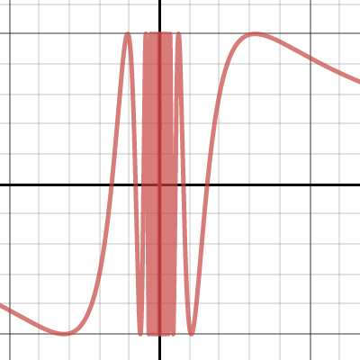
Does \(\lim_{x \to 0} \sin \left(\frac{1}{x}\right)\) exist?

Computational Approach

Let’s look at values of \(\sin(1/x)\) as \(x\) approaches 0.

x	sin(1/x)	x	sin(1/x)
\(1/\pi\)	0	\(2/\pi\)	1
\(1/(2\pi)\)	0	\(2/(5\pi)\)	\(\approx 0.58\)
\(1/(3\pi)\)	0	\(2/(9\pi)\)	\(\approx -0.98\)
\(1/(4\pi)\)	0	\(2/(13\pi)\)	\(\approx 0.74\)
\(1/(5\pi)\)	0	\(2/(17\pi)\)	\(\approx -0.99\)

As \(x\) approaches 0, \(f(x)\) does not settle on a single value; it oscillates infinitely between -1 and 1.

Graphical Approach

Graph of \(y = \sin(1/x)\)

The graph oscillates wildly near \(x=0\), never settling to a single y-value.

Warning

Since \(f(x)\) does not approach a single real number as \(x \to 0\), the limit \(\lim_{x \to 0} \sin \left(\frac{1}{x}\right)\) does not exist.

This example demonstrates a function where the limit does not exist.

The function ‘sin(1/x)’ is a classic example of oscillatory behavior near a point.

Computationally: If we choose values of x such that 1/x is a multiple of pi, like 1/pi, 1/(2pi), 1/(3pi), the sine of these values will always be 0. However, if we choose values such that 1/x is pi/2, 5pi/2, 9pi/2, the sine will be 1. And if 1/x is 3pi/2, 7pi/2, the sine will be -1. As x approaches 0, 1/x grows infinitely large, causing the sine function to cycle through all values between -1 and 1 infinitely many times.

Graphically: The image clearly shows this erratic oscillation. The graph literally cannot be drawn near x=0 as a continuous line to a single point. It’s impossible to pick one y-value that the function “approaches”.

This means there is no unique ‘L’ that ‘f(x)’ approaches, and therefore, the limit does not exist. This is a very important concept to grasp: just because a function is defined near a point doesn’t guarantee a limit exists.

4.2 One-sided Limit of a Function at a Point

Consider the function: \[ f (x) = \left\{ \begin{array}{cc} - 1 & x < 2 \\ 1 & x \geq 2 \end{array} \right. \] Is there a real number where \(f(x)\) approaches as \(x\) approaches 2?

Approaching from the Left (x < 2)

x	f(x)
0.5	-1
1.9	-1
1.99	-1
1.999	-1
1.9999	-1

As \(x \to 2\) from the left, \(f(x) \to -1\). We write this as: \[\lim_{x \to 2^-} f(x) = -1\] This is the Left-hand Limit.

Approaching from the Right (x > 2)

x	f(x)
2.5	1
2.1	1
2.01	1
2.001	1
2.0001	1

As \(x \to 2\) from the right, \(f(x) \to 1\). We write this as: \[\lim_{x \to 2^+} f(x) = 1\] This is the Right-hand Limit.

Warning

Since \(\lim_{x \to 2^-} f(x) \neq \lim_{x \to 2^+} f(x)\), the limit \(\lim_{x \to 2} f(x)\) does not exist. There is no single value \(f(x)\) approaches as \(x \to 2\).

One-sided limits are crucial for understanding function behavior at points where a function might “jump” or be defined differently on either side.

In this example, we have a piecewise function, a “Heaviside-like” step function. If we consider x values less than 2, the function is always -1. So, as x approaches 2 from the left, the function’s value remains -1. This is our left-hand limit.

Conversely, if we consider x values greater than or equal to 2, the function is always 1. So, as x approaches 2 from the right, the function’s value remains 1. This is our right-hand limit.

Since the left-hand limit (-1) is not equal to the right-hand limit (1), the overall limit as x approaches 2 does not exist. The function “jumps” at x=2.

Equal One-sided Limits

The following theorem connects the existence of a general limit to its one-sided counterparts.

Tip

Theorem 4.2.2 (Equal One-sided Limits)

\(\lim_{x \to a} f(x) = L\) if and only if \(\lim_{x \to a^-} f(x) = L\) and \(\lim_{x \to a^+} f(x) = L\).

Remark: This result is extremely useful for evaluating limits at a point \(a\) if the function has different mathematical expressions for \(x < a\) and \(x > a\) when \(x\) is near \(a\).

Equal One-sided Limits

Example: Let \(g(x) = \left\{ \begin{array}{ll} x^2 & \text{if } 0 < x \leq 1 \\ 0.5 & \text{if } x = 0 \\ \sin x & \text{if } -1 \leq x < 0 \end{array} \right.\) Does \(\lim_{x \to 0} g(x)\) exist?

Left-hand limit: \(\lim_{x \to 0^-} g(x) = \lim_{x \to 0^-} \sin x = \sin(0) = 0\).

Right-hand limit: \(\lim_{x \to 0^+} g(x) = \lim_{x \to 0^+} x^2 = (0)^2 = 0\).

Since \(\lim_{x \to 0^-} g(x) = 0\) and \(\lim_{x \to 0^+} g(x) = 0\), both one-sided limits are equal to 0.

Therefore, by Theorem 4.2.2, \(\lim_{x \to 0} g(x) = 0\).

This theorem provides a formal way to determine if a limit exists by examining its behavior from both sides. It states that a limit exists if and only if both the left-hand limit and the right-hand limit exist and are equal to the same value, L.

This is particularly important for piecewise functions, where the function’s definition changes at a specific point.

In the example, we evaluate the left-hand limit using the ‘sin x’ definition because that applies for x values less than 0. The right-hand limit uses the ‘x-squared’ definition for x values greater than 0. Both limits yield 0.

Since both one-sided limits are 0, the overall limit as x approaches 0 exists and is also 0. Notice that ‘g(0)’ is defined as 0.5, but this value does not affect the existence or value of the limit itself, only the continuity, which we’ll discuss later.

4.3 Infinite Limit

Let \(f\) be a function defined on both sides of \(a\), except possibly at \(a\) itself.

We write \(\lim_{x \to a} f(x) = \infty\) (or \(f(x) \to \infty\) as \(x \to a\)) if the values of \(f(x)\) can be made arbitrarily large (as large as we like) by taking \(x\) sufficiently close to \(a\) (but not equal to \(a\)).

Similarly, \(\lim_{x \to a} f(x) = -\infty\) means \(f(x)\) can be made arbitrarily negatively large.

4.3 Infinite Limit

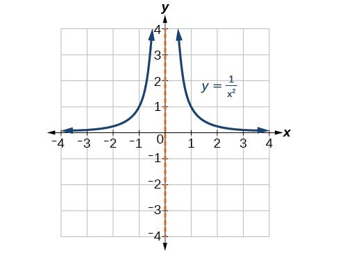
Example 4.3.1: What is \(\lim_{x \to 0} \frac{1}{x^2}\)?

Let’s evaluate \(f(x) = \frac{1}{x^2}\) for small values of \(x\):

x	f(x)	x	f(x)
0.1	100	-0.1	100
0.01	10,000	-0.01	10,000
0.001	1,000,000	-0.001	1,000,000
0.0001	10^8	-0.0001	10^8

As \(x\) becomes close to 0, \(\frac{1}{x^2}\) becomes very large.

Graph of \(y = 1/x^2\)

The graph shows that as \(x\) approaches 0 from either side, \(y\) increases without bound.

Note

The limit \(\lim_{x \to 0} \frac{1}{x^2}\) technically does not exist in terms of a finite real number. However, to describe this specific “blow-up” behavior, we write: \[\lim_{x \to 0} \frac{1}{x^2} = \infty\]

Infinite limits describe situations where a function’s value grows without bound (to positive or negative infinity) as the input approaches a certain point.

For the function ‘1/x^2’, as x gets very close to 0, whether from the positive or negative side, x^2 becomes a very small positive number. Dividing 1 by a very small positive number results in a very large positive number.

The computational table clearly shows this: as x approaches 0, f(x) grows rapidly. The graph visually confirms this, with the branches of the hyperbola shooting upwards as they get closer to the y-axis.

It’s important to remember that when we say a limit is infinity, we are technically stating that the limit does not exist in the sense of being a finite real number. However, using \(\infty\) or \(-\infty\) provides more specific information about how the limit fails to exist. This behavior is often associated with vertical asymptotes.

Vertical Asymptotes

The vertical line \(x = a\) is called a vertical asymptote of the curve \(y = f(x)\) if at least one of the following statements is true:

\[ \begin{array}{lll} \lim_{x \to a} f(x) = \infty & \lim_{x \to a^-} f(x) = \infty & \lim_{x \to a^+} f(x) = \infty \\ \lim_{x \to a} f(x) = -\infty & \lim_{x \to a^-} f(x) = -\infty & \lim_{x \to a^+} f(x) = -\infty \end{array} \]

Vertical Asymptotes

Examples of Vertical Asymptotes:

1. The vertical line with equation \(x = 0\) (the \(y\)-axis) is a vertical asymptote of \(y = \frac{1}{x^2}\).

(As seen in the previous slide, \(\lim_{x \to 0} \frac{1}{x^2} = \infty\))

2. The lines \(x = \pm \frac{\pi}{2}\) are vertical asymptotes of the curve \(y = \tan x\).

(Think about the unit circle or the graph of tangent; it “blows up” at these points)

3. The vertical line \(x = 0\) is a vertical asymptote of \(y = \ln x\).

(The natural logarithm is only defined for \(x>0\), and as \(x \to 0^+\), \(\ln x \to -\infty\))

Graph of \(y = \tan x\)

Vertical asymptotes are vertical lines that a function’s graph approaches but never touches, as the function’s value tends towards positive or negative infinity. They are directly related to infinite limits.

If any of the six conditions listed are met, then x=a is a vertical asymptote. This means that if the function “blows up” to positive or negative infinity as x approaches ‘a’ from either or both sides, then we have a vertical asymptote.

Review the examples: (a) For 1/x^2, as discussed, the function goes to positive infinity from both sides of x=0. (b) For tan x, the tangent function is sin x / cos x. When cos x is zero (at pi/2, 3pi/2, etc.), the function becomes undefined and shoots off to infinity or negative infinity. (c) For ln x, its domain is x > 0. As x approaches 0 from the right side, ln x goes to negative infinity. This shows a one-sided infinite limit can also define a vertical asymptote.

Understanding vertical asymptotes is crucial for sketching graphs and analyzing the behavior of functions.

4.4 Limits at Infinity

Let \(f(x)\) be a function defined on some interval \((a, \infty)\) (for large positive \(x\)) or \((-\infty, a)\) (for large negative \(x\)).

We write \(\lim_{x \to \infty} f(x) = L\) (or \(\lim_{x \to -\infty} f(x) = L\)) if the values of \(f(x)\) can be made as close to \(L\) as we like by taking \(x\) sufficiently large (or sufficiently negatively large).

4.4 Limits at Infinity

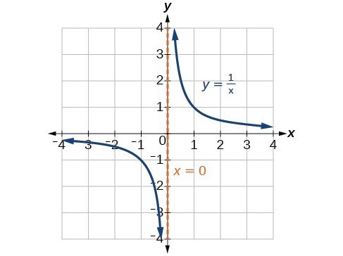
Example 4.4.1: For the function \(f(x) = \frac{1}{x}\), what happens to the values of \(f(x)\) as \(x\) increases to large positive values?

x	f(x)
10	0.1
100	0.01
1,000	0.001
10,000	0.0001
…	…
\(10^N\)	\(10^{-N}\)

As \(x \to \infty\), \(f(x)\) approaches 0. \[\lim_{x \to \infty} \frac{1}{x} = 0\]

Graph of \(y = 1/x\)

The graph shows that as \(x\) gets very large (positive or negative), \(y\) approaches 0. Similarly, \(\lim_{x \to -\infty} \frac{1}{x} = 0\).

Limits at infinity describe the end behavior of a function—what happens to the function’s output as the input ‘x’ grows infinitely large in either the positive or negative direction.

For ‘f(x) = 1/x’, as x takes on larger and larger positive values (e.g., 10, 100, 1000), the fraction 1/x becomes smaller and smaller, getting closer to 0. It never actually reaches 0, but it gets arbitrarily close.

The graph visually confirms this: as you move far to the right along the x-axis, the curve gets closer and closer to the x-axis (y=0). The same happens when x goes to negative infinity.

If a function approaches a finite value ‘L’ as ‘x’ approaches infinity (either positive or negative), then the line y=L is a horizontal asymptote. This gives us crucial information about the shape of the graph far away from the origin.

Horizontal Asymptotes

The horizontal line \(y = b\) is called a horizontal asymptote of the curve \(y = f(x)\) if:

\[ \lim_{x \to \infty} f(x) = b \quad \text{or} \quad \lim_{x \to -\infty} f(x) = b. \]

Examples of Horizontal Asymptotes:

1. For every positive integer \(n\), note that \(\lim_{x \to \infty} \frac{1}{x^n} = 0\), and \(\lim_{x \to -\infty} \frac{1}{x^n} = 0\).

The horizontal line \(y = 0\) (the \(x\)-axis) is a horizontal asymptote of \(y = \frac{1}{x^n}\).

2. Note that \(\lim_{x \to -\infty} e^x = 0\). The horizontal line \(y = 0\) is a horizontal asymptote of the curve \(y = e^x\).

(As \(x\) goes to positive infinity, \(e^x\) goes to infinity, so no horizontal asymptote there)

3. The following limits at infinity do not exist as finite numbers: \(\lim_{x \to \infty} \sin x\), \(\lim_{x \to \infty} \cos x\), \(\lim_{x \to \infty} \tan x\), \(\lim_{x \to \infty} e^x\), \(\lim_{x \to \infty} \ln x\).

(These functions either oscillate, grow infinitely large, or are undefined for large negative values)

4. Inverse tangent has horizontal asymptotes: \(\lim_{x \to \infty} \tan^{-1} x = \frac{\pi}{2}\) \(\lim_{x \to -\infty} \tan^{-1} x = -\frac{\pi}{2}\) So, \(y = \frac{\pi}{2}\) and \(y = -\frac{\pi}{2}\) are horizontal asymptotes.

Horizontal asymptotes describe the behavior of a function as its input ‘x’ becomes extremely large (positive or negative). If the function’s output ‘f(x)’ approaches a specific finite value ‘b’ in these extreme cases, then ‘y=b’ is a horizontal asymptote.

It’s possible for a function to have one, two, or no horizontal asymptotes.

For ‘1/x^n’, as x gets very large, the denominator grows, making the fraction approach 0. So y=0 is a horizontal asymptote.

For ‘e^x’, as x goes to negative infinity, e^x approaches 0. However, as x goes to positive infinity, e^x grows without bound, so there’s no horizontal asymptote in that direction.

Functions like sin x and cos x oscillate, so they don’t approach a single value at infinity. The inverse tangent function, however, clearly demonstrates two distinct horizontal asymptotes as x approaches positive and negative infinity. This is a good example of a function having two different horizontal asymptotes.

4.5 Limit Theorems

Limit laws simplify the evaluation of complex limits by breaking them down into simpler components.

Important

Theorem 4.5.1 (Basic Limits)

1. \(\lim_{x \to a} C = C\)
2. \(\lim_{x \to a} x = a\)

Theorem 4.5.2 (Arithmetic of Limits)

1. \(\lim_{x \to a} Cf(x) = C \lim_{x \to a} f(x)\)
2. \(\lim_{x \to a} (f(x) \pm g(x)) = \lim_{x \to a} f(x) \pm \lim_{x \to a} g(x)\)

Example 4.5.3:

1. \(\lim_{x \to \pi} 7x = 7 \lim_{x \to \pi} x = 7\pi\)
2. \(\lim_{x \to \pi} (7x + \sqrt{3}) = \lim_{x \to \pi} 7x + \lim_{x \to \pi} \sqrt{3} = 7\pi + \sqrt{3}\)

These theorems, often called “limit laws,” are extremely powerful. They allow us to evaluate limits of combinations of functions if we know the limits of the individual functions.

Theorem 4.5.1 establishes the most basic limits: the limit of a constant is the constant itself, and the limit of ‘x’ as ‘x’ approaches ‘a’ is ‘a’. These are intuitively clear.

Theorem 4.5.2 provides rules for scalar multiplication, addition, and subtraction of functions. We can pull constants out of limits, and we can distribute the limit operator over sums and differences.

The examples illustrate how these rules are applied step-by-step. This systematic approach is the foundation for evaluating more complex limits. Remember, these laws are valid provided the individual limits on the right-hand side exist.

More Limit Laws

Important

Theorem 4.5.4 (Product and Power Laws)

3. \(\lim_{x \to a} f(x)g(x) = \lim_{x \to a} f(x) \cdot \lim_{x \to a} g(x)\)
4. \(\lim_{x \to a} (f(x))^n = (\lim_{x \to a} f(x))^n\), where \(n\) is a positive integer.

Example 4.5.5:

3. \(\lim_{x \to \pi} (7x)(x) = \lim_{x \to \pi} (7x) \cdot \lim_{x \to \pi} (x) = (7\pi)(\pi) = 7\pi^2.\)
4. \(\lim_{x \to a} (x)^n = (\lim_{x \to a} x)^n = a^n\), where \(n\) is a positive integer.

Important

Theorem 4.5.6 (Quotient Law)

5. \(\lim_{x \to a} \frac{f(x)}{g(x)} = \frac{\lim_{x \to a} f(x)}{\lim_{x \to a} g(x)},\) if \(\lim_{x \to a} g(x) \neq 0\).

Example 4.5.7:

5. \(\lim_{x \to \pi} \frac{7}{x^3} = \frac{\lim_{x \to \pi} 7}{\lim_{x \to \pi} x^3} = \frac{7}{\pi^3},\) since \(\lim_{x \to \pi} x^3 = \pi^3 \neq 0\).

Tip

All the above Limit Laws hold for one-sided limits (\(\lim_{x \to a^+}\), \(\lim_{x \to a^-}\)) and limits at infinity (\(\lim_{x \to \infty}\), \(\lim_{x \to -\infty}\)).

Continuing with limit laws, these theorems cover products, powers, and quotients of functions.

Theorem 4.5.4 allows us to find the limit of a product of functions by multiplying their individual limits. It also states that we can take the limit of a function raised to a positive integer power by taking the limit of the function first and then raising it to that power.

Theorem 4.5.6 is for quotients. It states that the limit of a quotient of two functions is the quotient of their limits, provided that the limit of the denominator is not zero. This is a critical condition; if the denominator’s limit is zero, we cannot use this law directly, and other techniques might be needed.

The examples illustrate the application of these laws. The final tip reminds us that these powerful laws are not restricted to two-sided limits at a finite point; they extend to one-sided limits and limits at infinity, which is very convenient.

Limits of Polynomials and Rational Functions

Limits of a Polynomial

Important

Theorem 4.5.9: For a polynomial \(p(x) = a_n x^n + a_{n-1} x^{n-1} + \dots + a_1 x + a_0\),

we have \(\lim_{x \to a} p(x) = p(a)\).

This means we can simply substitute the value of \(a\) into the polynomial \(p(x)\) to obtain the limit of \(p(x)\) at \(a\).

Example 4.5.10:

\(\lim_{x \to 1}\left(2x^5 -\pi x^3 +\frac{1}{9} x - \sqrt{5}\right) = 2(1)^5 - \pi(1)^3 + \frac{1}{9}(1) - \sqrt{5} = 2 - \pi +\frac{1}{9} -\sqrt{5}.\)

Limits of Polynomials and Rational Functions

Rational Functions

A function \(f(x)\) is a rational function if it is a quotient of two polynomials, i.e., \(f(x) = \frac{p(x)}{q(x)}\).

Important

Theorem 4.5.11: If \(f(x) = \frac{p(x)}{q(x)}\) and \(a\) is such that \(q(a) \neq 0\), then: \[ \lim_{x \to a} \frac{p(x)}{q(x)} = \frac{p(a)}{q(a)}. \]

Again, we can simply substitute \(a\) into the function, provided the denominator is not zero.

Example 4.5.12:

Evaluate \(\lim_{x \to 3}\frac{3x + 6}{x^2 - 4}\).
Here, \(p(x) = 3x+6\) and \(q(x) = x^2-4\).
Since \(q(3) = 3^2 - 4 = 9 - 4 = 5 \neq 0\), we can substitute:
\(\lim_{x \to 3}\frac{3x + 6}{x^2 - 4} = \frac{3(3) + 6}{3^2 - 4} = \frac{9 + 6}{9 - 4} = \frac{15}{5} = 3\).

These two theorems are incredibly helpful because they simplify limit calculations for two common types of functions: polynomials and rational functions.

For any polynomial, the limit as x approaches ‘a’ is simply the value of the polynomial at ‘a’. This is a direct consequence of the limit laws we just discussed. You can just plug in the value!

For rational functions (a ratio of two polynomials), you can also substitute ‘a’ directly, but only if the denominator is not zero at ‘a’. This is a crucial condition. If the denominator is zero, direct substitution leads to an indeterminate form (like 0/0) or an infinite limit (like L/0), and other techniques are required.

The warning about substitution failing is very important to remember. Direct substitution is a shortcut, but it only works when certain conditions are met, namely, when the function is continuous at that point (a concept we’ll fully define next).

Substitution May Fail!

We cannot apply direct substitution to find limits like: \[ \lim_{x \to 3} \frac{x^2 - 2x - 3}{x^2 - 9} \] Why?

Because if we substitute \(x=3\) into the denominator, we get \(3^2 - 9 = 9 - 9 = 0\).

Similarly, substituting \(x=3\) into the numerator gives \(3^2 - 2(3) - 3 = 9 - 6 - 3 = 0\).

This gives us the indeterminate form \(\frac{0}{0}\).

Warning

In general, we cannot simply substitute values of \(a\) directly into the function \(f(x)\) to obtain the limit of \(f(x)\) at \(a\). Such substitution holds when the functions involved are continuous at \(a\). We shall discuss this concept of continuity in the next section.

This slide emphasizes a critical point: direct substitution is not always valid. The theorems for polynomials and rational functions provide shortcuts, but they have conditions.

When direct substitution leads to an indeterminate form like 0/0, it means that the limit cannot be found by simply plugging in the value. This form indicates that there might still be a limit, but we need to employ other techniques (like algebraic simplification, factorization, or rationalization) to find it.

The warning foreshadows the next section on continuity. The ability to substitute directly is a hallmark of continuous functions. If a function is continuous at a point, its limit at that point is simply its function value at that point. If a function is not continuous at that point (e.g., due to a hole or a jump), direct substitution might fail or give an incorrect result for the limit.

4.6 Continuity

Most functions you’ve encountered in pre-university math are “nice” in the sense that their graphs are continuous.

Such functions allow us to substitute the value \(c\) directly into \(f(x)\) to evaluate \(\lim_{x \to c} f(x)\).

This “niceness” has a mathematical name: continuity at \(x = c\).

4.6 Continuity

Continuity at a Point

Important

Definition 4.6.1 (Continuity at a Point)

Let \(f\) be a function defined on an interval \(I\) and let \(c\) be an interior point of \(I\). We say that \(f\) is continuous at \(x = c\) if \[ \lim_{x \to c} f(x) = f(c). \]

In words, this definition means three things must be true for \(f\) to be continuous at \(x = c\):

1. \(f(c)\) is defined. The function must have a value at \(c\).
2. \(\lim_{x \to c} f(x)\) exists. The limit as \(x\) approaches \(c\) must be a finite number.
3. \(\lim_{x \to c} f(x) = f(c)\). The limit must be equal to the function’s value at \(c\).

Tip

Continuity at \(x=c\) means we can interchange the order of “lim” and “f”:

\(\lim_{x \to c} f(x) = f(\lim_{x \to c} x) = f(c)\).

Continuity is a fundamental concept in calculus, essentially meaning a function’s graph can be drawn without lifting your pencil. No breaks, no jumps, no holes.

The formal definition ties together the concepts of limits and function values. For a function to be continuous at a point ‘c’, three conditions must be met simultaneously:

1. The function must have a value at ‘c’ (no holes or undefined points).
2. The limit of the function as x approaches ‘c’ must exist (no jumps or wild oscillations).
3. The limit value must be equal to the function value (the hole must be filled in exactly by the function’s value at that point).

If any of these three conditions fail, the function is not continuous at ‘c’. The tip highlights the practical implication: if a function is continuous, direct substitution for limits works!

Basic Functions and Their Limits

Many common functions are continuous on their natural domains.

Note

Basic Functions Continuous on their Domains:

Polynomials, rational functions (where denominator \(\neq 0\)), \(\sqrt[n]{x}\), \(\sin x\), \(\cos x\), \(\tan x\) (where defined), \(e^x\), and \(\ln x\) (where defined) are continuous at every point in their domain.

Limits of Basic Functions (Theorem 4.6.3)

Since these functions are continuous, their limits can be found by direct substitution:

1. \(\lim_{x \to c}\sqrt[n]{x} = \sqrt[n]{c}\) (for \(n\) odd, \(c \in \mathbb{R}\); for \(n\) even, \(c > 0\))
2. \(\lim_{x \to c}\sin x = \sin c\)
3. \(\lim_{x \to c}\cos x = \cos c\)
4. \(\lim_{x \to c}\tan x = \tan c\) (where \(\tan c\) is defined)
5. \(\lim_{x \to c} b^x = b^c\) for any \(b > 0\); in particular, \(\lim_{x \to c} e^x = e^c\).
6. \(\lim_{x \to c}\ln x = \ln c\) (where \(c > 0\))
7. \(\lim_{x \to c}\sinh x = \sinh c\)
8. \(\lim_{x \to c}\cosh x = \cosh c\)
9. \(\lim_{x \to c}\tanh x = \tanh c\)
10. Inverse trigonometric and hyperbolic functions are continuous at \(c\) (not endpoints).

Example 4.6.2:

1. \(f(x) = \sin x\) is continuous for each \(x \in \mathbb{R}\).
2. \(g(x) = \ln x\) is continuous for each \(x \in (0, \infty)\).
3. \(h(x) = \tan x\) is continuous for each \(x \in \mathbb{R} \setminus \{ \frac{\pi}{2} + k\pi \mid k \in \mathbb{Z} \}\).

This slide compiles a list of common functions that are inherently continuous within their domains. This is extremely useful because it means for any point within their domain, you can find the limit simply by plugging in the value, thanks to the definition of continuity.

For instance, ‘sin x’ is continuous everywhere. So, if you want to find the limit of ‘sin x’ as x approaches pi/2, it’s just ‘sin(pi/2) = 1’. No need for complex limit calculations.

However, it’s important to be mindful of the domains. For ‘ln x’, it’s continuous only for positive x values. For ‘tan x’, it’s continuous everywhere except where cosine is zero (i.e., at odd multiples of pi/2), which are its vertical asymptotes.

Understanding the continuity of these basic functions simplifies many limit problems and forms a building block for understanding more complex function behavior.

Test for Continuity - Examples

To check if a function \(f\) is continuous at \(x = c\), we must verify all three conditions:

1. \(f(c)\) is defined.
2. \(\lim_{x \to c} f(x)\) exists.
3. \(f(c) = \lim_{x \to c} f(x)\).

Example 4.6.4:

Consider \(f(x) = \frac{1 - x^2}{1 - x}\). Is \(f\) continuous at \(x = 1\)?

1. \(f(1)\) is defined? No, \(f(1) = \frac{0}{0}\) (undefined).

   Therefore, \(f\) is not continuous at \(x = 1\).

   (Note: We previously found \(\lim_{x \to 1} f(x) = 2\), so (ii) exists, but (i) fails.)

Test for Continuity - Examples

Example 4.6.5:

Let \(f: \mathbb{R} \to \mathbb{R}\) be defined by \(f(x) = \left\{ \begin{array}{ll} 1 & \text{for } x = 2 \\ 0 & \text{for } x \neq 2 \end{array} \right.\). Is \(f\) continuous at \(x = 2\)?

1. \(f(2)\) is defined? Yes, \(f(2) = 1\).

2. \(\lim_{x \to 2} f(x)\) exists?

   As \(x \to 2\) from left or right, \(x \neq 2\), so \(f(x) = 0\). Thus, \(\lim_{x \to 2} f(x) = 0\).

3. \(f(2) = \lim_{x \to 2} f(x)\)? No, \(1 \neq 0\).

   Therefore, \(f\) is not continuous at \(x = 2\). This is a removable discontinuity (a “point discontinuity”).

Example 4.6.6:

Let \(f(x) = \left\{ \begin{array}{ll} \sin \frac{1}{x} & \text{for } x \neq 0 \\ 1 & \text{for } x = 0 \end{array} \right.\). Is \(f\) continuous at \(x = 0\)?

1. \(f(0)\) is defined? Yes, \(f(0) = 1\).

2. \(\lim_{x \to 0} f(x)\) exists? No, as seen before, \(\lim_{x \to 0} \sin \frac{1}{x}\) does not exist.

   Therefore, \(f\) is not continuous at \(x = 0\). This is an oscillating discontinuity.

These examples illustrate how the three conditions for continuity at a point are applied and how a function can fail to be continuous.

In Example 4.6.4, ‘f(1)’ is undefined. This is the simplest way for continuity to fail – there’s a hole in the graph. Even though the limit exists, the function value is missing.

In Example 4.6.5, ‘f(2)’ is defined, and the limit as x approaches 2 exists and is 0. However, the function value at 2 (which is 1) does not match the limit (which is 0). The graph has an isolated point at (2,1) while the rest of the function approaches (2,0). This is called a removable discontinuity, as you could “fix” it by redefining f(2) to be 0.

In Example 4.6.6, ‘f(0)’ is defined, but the limit itself does not exist due to the wild oscillation of ‘sin(1/x)’ near 0. This is a more complex type of discontinuity.

Understanding these different ways continuity can fail helps in classifying and analyzing function behavior.

4.7 One-sided Continuity

Sometimes, a function is continuous only from one side at a boundary point of its domain.

Important

Definition 4.7.1 (One-sided Continuity)

• We say that \(f\) is continuous from the left at \(x = c\) if \(\lim_{x \to c^-} f(x) = f(c)\).
• We say that \(f\) is continuous from the right at \(x = c\) if \(\lim_{x \to c^+} f(x) = f(c)\).

4.7 One-sided Continuity

Example 4.7.2: Discuss the continuity of the Heaviside function \(H\) at \(x = 0\): \[ H(x) = \left\{ \begin{array}{ll} 0 & \text{for } x < 0 \\ 1 & \text{for } x \geq 0 \end{array} \right. \]

1. \(H(0)\) is defined? Yes, \(H(0) = 1\).
2. \(\lim_{x \to 0} H(x)\) exists?
   • \(\lim_{x \to 0^-} H(x) = \lim_{x \to 0^-} 0 = 0\).
   • \(\lim_{x \to 0^+} H(x) = \lim_{x \to 0^+} 1 = 1\). Since \(0 \neq 1\), \(\lim_{x \to 0} H(x)\) does not exist.

Therefore, \(H(x)\) is not continuous at \(x = 0\).

One-sided continuity check:

• Continuous from the right? \(\lim_{x \to 0^+} H(x) = 1\) and \(H(0) = 1\). Since \(\lim_{x \to 0^+} H(x) = H(0)\), \(H\) is continuous from the right at \(x = 0\).

• Continuous from the left? \(\lim_{x \to 0^-} H(x) = 0\) and \(H(0) = 1\). Since \(\lim_{x \to 0^-} H(x) \neq H(0)\), \(H\) is not continuous from the left at \(x = 0\).

One-sided continuity extends the concept of continuity to include points at the boundaries of an interval, or at points where a function might have a “jump” discontinuity.

The Heaviside function is a perfect example of a function that is continuous from one side but not the other.

At x=0: 1. The function value H(0) is 1. 2. The left-hand limit is 0, and the right-hand limit is 1. Since these are not equal, the overall limit at x=0 does not exist, and thus the function is not generally continuous at x=0.

However, when we check one-sided continuity: - From the right, the limit is 1, and the function value is 1. They match! So, the Heaviside function is continuous from the right at x=0. - From the left, the limit is 0, but the function value is 1. They do not match. So, it’s not continuous from the left at x=0.

This illustrates a “jump discontinuity,” where the function literally jumps from one value to another at a specific point.

4.8 Properties of Continuity

Just like limit laws, continuity has properties that apply to combinations of functions.

Important

If \(f\) and \(g\) are continuous at \(x = c\), then the following combinations are also continuous at \(x = c\):

1. \(f \pm g\) (sum or difference)
2. \(f \cdot g\) (product)
3. \(f / g\) (quotient, provided \(g(c) \neq 0\))

Proof Sketch (for Sum/Difference): \[ \begin{aligned} \lim_{x \to c} (f \pm g)(x) &= \lim_{x \to c} f(x) \pm \lim_{x \to c} g(x) & \text{(by Limit Law 2)} \\ &= f(c) \pm g(c) & \text{(since } f, g \text{ are continuous at } c) \\ &= (f \pm g)(c) & \text{(by definition of sum/difference)} \end{aligned} \] This matches the definition of continuity at \(c\).

4.8 Properties of Continuity

Example 4.8.1:

Evaluate \(\lim_{x \to 1}\left(x^{-2} - 4x^{1 / 7} - 5x^5 +\sqrt{2} x + \pi\right)\).

Each term (\(x^{-2}\), \(4x^{1/7}\), \(5x^5\), \(\sqrt{2}x\), \(\pi\)) is continuous at \(x = 1\).

Therefore, the entire function (a sum/difference of continuous functions) is continuous at \(x = 1\).

So, we can evaluate by direct substitution: \[ \begin{aligned} &= 1^{-2} - 4(1^{1/7}) - 5(1^5) + \sqrt{2}(1) + \pi \\ &= 1 - 4 - 5 + \sqrt{2} + \pi \\ &= -8 + \sqrt{2} + \pi. \end{aligned} \]

These properties of continuity are direct consequences of the limit laws. They make it much easier to determine the continuity of complex functions built from simpler, known continuous functions.

If you have two functions, ‘f’ and ‘g’, that are continuous at a specific point ‘c’, then their sum, difference, and product will also be continuous at ‘c’. For their quotient to be continuous, we need the additional condition that the denominator ‘g(c)’ is not zero.

The proof sketch demonstrates how the limit laws directly lead to the continuity properties. The ability to swap the limit and the function operation is precisely what continuity allows.

The example shows the practical application: because each individual term in the expression is continuous at x=1, their sum/difference is also continuous. This means we can evaluate the limit by simply plugging in x=1, simplifying the calculation significantly.

Limit Law for Composite Functions

The limit law for composite functions requires the outermost function to be continuous.

Important

Theorem 4.8.2 (Limit of Composite Functions)

Suppose that \(\lim_{x \to c} g(x) = b\) and \(f\) is continuous at \(b\).

Then \[ \lim_{x \to c} f(g(x)) = \lim_{y \to b} f(y) = f(b). \] That is, \(\lim_{x \to c} f(g(x)) = f\left(\lim_{x \to c} g(x)\right) = f(b)\).

This theorem says we can interchange the order of taking the limit and applying the function \(f\) (we can “bring the limit inside” \(f(\cdot)\)).

Corollary 4.8.3 (Applications):

1. \(\lim_{x \to c}\sqrt[n]{g(x)} = \sqrt[n]{\lim_{x \to c}g(x)}\)
2. \(\lim_{x \to c} e^{g(x)} = e^{\lim_{x \to c} g(x)}\)

Limit Law for Composite Functions

Example 4.8.4:

The following functions are continuous at the specified \(x = c\). Hence, the limits can be evaluated by direct substitution.

1. \(\lim_{x \to 7}\sqrt[3]{x + 20}\cos \left(\frac{\pi x}{2}\right)\)
   • Here, \(g(x) = x+20\) and \(f(y) = \sqrt[3]{y}\). Also \(h(x) = \frac{\pi x}{2}\) and \(k(y) = \cos y\). Both \(\sqrt[3]{y}\) and \(\cos y\) are continuous everywhere.
   • \(\lim_{x \to 7}(x+20) = 27\) and \(\lim_{x \to 7}(\frac{\pi x}{2}) = \frac{7\pi}{2}\).
   • So, \(\lim_{x \to 7}\sqrt[3]{x + 20}\cos \left(\frac{\pi x}{2}\right) = \sqrt[3]{27}\cos \left(\frac{7\pi}{2}\right) = 3 \cdot 0 = 0\).
2. \(\lim_{x \to e^2}\frac{\sin(x - e^x)}{\ln x}\)
   • The numerator \(\sin(x - e^x)\) is a composition of continuous functions (\(\sin y\) and \(x-e^x\)), so it’s continuous.
   • The denominator \(\ln x\) is continuous for \(x > 0\). At \(x = e^2\), \(\ln(e^2) = 2 \neq 0\).
   • So, by quotient rule, we can substitute directly: \(\frac{\sin(e^2 - e^{e^2})}{\ln(e^2)} = \frac{\sin(e^2 - e^{e^2})}{2}\).

The Limit Law for Composite Functions is another powerful tool. It essentially states that if you have a function nested inside another function (a composite function), and the outer function is continuous, then you can “move” the limit inside the outer function.

This simplifies many limit evaluations, particularly for functions involving roots, exponentials, logarithms, and trigonometric functions applied to an inner function whose limit is known.

The corollaries are specific applications of this theorem, showing how it works for nth roots and exponential functions.

The examples demonstrate the chain of reasoning: identify the inner and outer functions, verify the continuity of the outer function at the limit of the inner function, and then apply the theorem by direct substitution. This makes what could be very complicated limits quite straightforward to calculate.