Machine Learning

CNN

Imron Rosyadi

Convolutional Neural Networks (CNNs)

Welcome to today’s lecture on Convolutional Neural Networks. We’ll explore how these powerful models have revolutionized computer vision, focusing on their architecture and underlying operations. As ECE students, understanding the engineering principles behind CNNs is crucial for designing and deploying advanced ML systems.

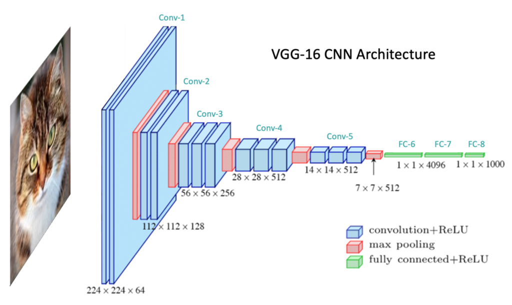
VGG-16 CNN

What We’ll Cover

1. Motivation: Why CNNs? - Limitations of traditional MLPs for images - Translation invariance & parameter efficiency

2. CNN Architecture Components - Feature Extractors & Classifiers - VGG-16 example

3. The Convolutional Block - Convolutional Layers: Filters, Kernels, Operations - Pooling Layers: Downsampling & regularization

4. The Fully Connected Classifier - Transforming features to probabilities

5. Advanced Topics & Summary - Dropout, Batch Normalization, 3D Convolutions

Our journey today will start by understanding the “why” behind CNNs, looking at the challenges traditional Multi-Layer Perceptrons face with image data. Then, we’ll dive into the fundamental building blocks of CNNs, specifically the convolutional and pooling layers, which form the feature extraction part. We’ll dissect the convolution operation itself, understanding concepts like filters, kernels, stride, and padding. After features are extracted, we’ll see how fully connected layers classify these features. Finally, we’ll touch upon some advanced techniques and summarize the key takeaways, ensuring we connect theory to practical application in ECE.

Motivation: Limitations of MLPs for Image Data

Traditional Fully Connected Networks (MLPs) struggle with image data.

1. Not Translation Invariant

• Main content shifted = different network output.
• Requires training on all possible shifts, which is inefficient.

Caution

MLPs treat each pixel as an independent feature. Spatial relationships are lost if features move.

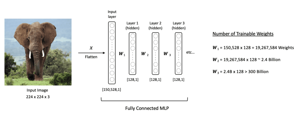
2. Prone to Overfitting (Parameter Explosion)

• Each input pixel connects to every neuron in the next layer.
• Example: 224x224x3 color image \(\rightarrow\) 150,528 input neurons.
• With just three modest hidden layers, parameters can exceed 300 Billion!

Tip

Large number of parameters makes training difficult and increases overfitting risk.

Not Translation Invariant

Prone to Overfitting

When we talk about image data, we’re dealing with spatial information. Think about a handwritten digit ‘7’. If it’s in the center of an image or slightly shifted to the left, it’s still a ‘7’. However, for a traditional MLP, if the ‘7’ shifts, the pixel values hitting the input neurons change dramatically, leading to a different internal representation, and potentially, a wrong classification without extensive training data for all possible shifts. This is what we mean by “not translation invariant”.

Secondly, images are high-dimensional. A seemingly small image like 224x224 pixels with 3 color channels has over 150,000 pixel values. If we link each of these to even a modest number of neurons in the next layer, the number of trainable weights explodes rapidly. This makes the network incredibly complex, slow to train, and highly susceptible to overfitting, where it memorizes the training data rather than learning generalizable features. This is where CNNs come in.

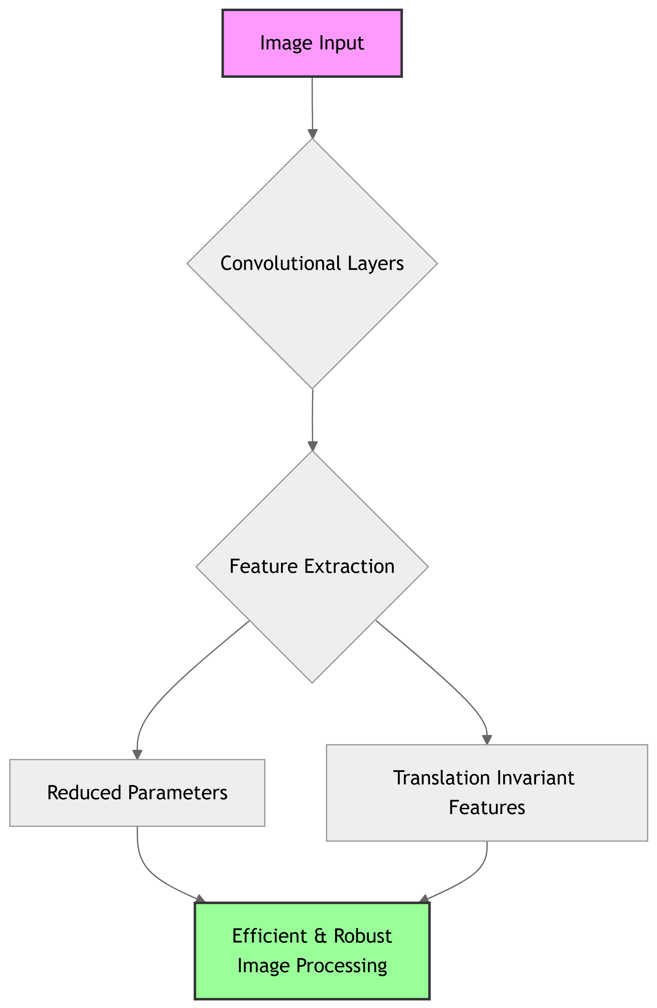
Convolutional Neural Networks (CNNs) to the Rescue!

CNNs are designed to efficiently process image data.

Key Features

• Convolution Operations: Extract features effectively.
• Parameter Sharing: Same weights process different input parts.
  • Greatly reduces total trainable parameters.
• Translation Invariance: Detect features regardless of position.
  • Kernel slides, detecting patterns like edges or textures.

Important

CNNs leverage local spatial coherence in images.

How CNNs Solve MLP Issues

VGG-16

Fortunately, CNNs provide a much more effective solution for image data. The core idea is the “convolution operation.” Instead of individual neurons looking at single pixels, small learnable filters, also called kernels, slide across the image. This parameter sharing means the same filter can detect a specific feature, like a vertical edge, anywhere in the image. This dramatically reduces the number of learnable parameters compared to an MLP. Because the filter slides, it inherently gives CNNs translation invariance. If an object shifts, the same filter will still activate when it encounters that object, just at a different location on its activation map. This leads to much more efficient and robust image processing models, a cornerstone of ECE applications in robotics, autonomous systems, and medical imaging.

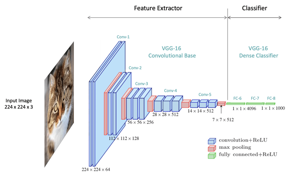
CNN Architecture: Feature Extractor & Classifier

Most CNNs follow a two-part structure:

1. Feature Extractor (Backbone)

• Purpose: Extract meaningful features from raw input.
• Comprises Convolutional Blocks (Conv + Activation + Pooling).
• Spatial dimensions are reduced, depth (channels) increased.
  • Example: Input (224x224x3) \(\rightarrow\) Features (7x7x512).

2. Classifier (Head)

• Purpose: Transform extracted features into class predictions.
• Typically uses Fully Connected (Dense) Layers.
• Final layer outputs probabilities (e.g., Softmax).

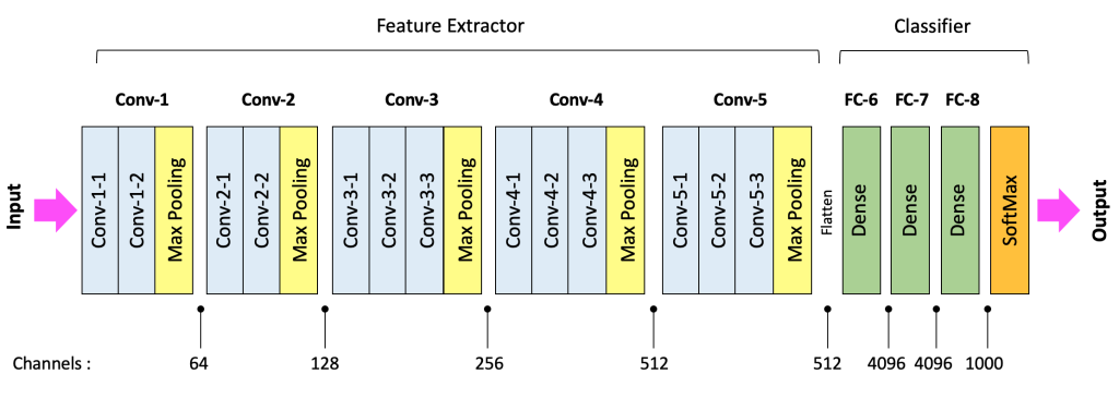
VGG-16 High-Level Architecture

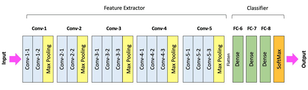
Feature Extractor and Classifier

A key concept in CNN architecture is the separation into a feature extractor and a classifier. The feature extractor, often called the “backbone,” is responsible for taking the raw input image and transforming it into a high-level representation of its features. This is done through a series of “convolutional blocks,” where each block typically involves convolutional layers followed by a pooling layer. As data flows through these blocks, the spatial dimensions of the data are typically reduced, while the ‘depth’ — or the number of channels — increases, representing more complex and abstract features. You can see this visually in the VGG-16 diagram, where the input starts as 224x224x3 and by ConvBlock5, it’s 7x7x512.

Once these features are extracted, the classifier, or “head,” takes over. It’s usually composed of one or more fully connected layers that take these abstract features and map them to probabilities for each possible output class. For VGG-16, trained on ImageNet, the output layer has 1000 neurons, each corresponding to one of the 1000 classes.

The Graphviz diagram on the right illustrates this high-level structure using the VGG-16 example. You can see the flow from raw image input, through the convolutional blocks, flattening the tensor, and finally through the fully connected layers to the final classification.

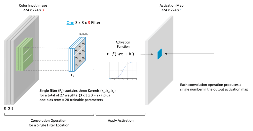
Convolutional Layers: The “Eyes” of a CNN

Extracting features using learnable filters.

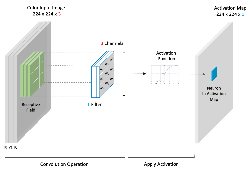
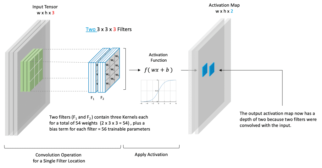
How it Works

1. Input: A 2D array (image or feature map).
2. Filter/Kernel: Small (e.g., 3x3) matrix of weights.
3. Convolution Operation:
   • Filter slides across input data.
   • At each position, element-wise multiplication & sum of filter and receptive field.
   • Result is a single number.
4. Activation Map: Output of the convolution, passed through an activation function.
   • Summarizes features from the input.

Conceptual Diagram

Note

Filter weights are learned during training. Unlike fixed filters (e.g., Sobel), CNN filters adapt for optimal feature detection.

Convolution Operation

The convolutional layer is the heart of a CNN. It’s often called the “eyes” because it’s where the network actually “looks” for patterns. Imagine you have an input image. A small window, called a filter or kernel, slides over this image. This filter contains a set of weights, which are initially random but become precisely tuned during the training process. At each position the filter lands, it performs an element-wise multiplication of its weights with the corresponding pixel values in the “receptive field” of the input. All these products are then summed up to produce a single number. This process is repeated as the filter slides, creating a new matrix called an activation map. This map essentially highlights where the feature that the filter is looking for is present in the input. Finally, this activation map usually undergoes a non-linear activation function, like ReLU, before being passed to the next layer. This non-linearity is crucial for the network to learn complex patterns.

Convolution Operation: Stride and Padding

Controlling the output size and feature detection.

Stride

• Definition: Number of pixels the filter shifts at a time.
• Stride 1: Filter moves one pixel at a time (most common).
• Stride > 1: Downsamples the output, reducing feature map size.
  • Learn fewer features, smaller output.

Tip

Adjusting stride allows control over spatial dimension reduction. A stride of 2 halves the spatial dimensions.

Padding

• Definition: Adding extra pixels (usually zeros) around input borders.
• Purpose:
  • Preserve spatial dimensions (e.g., input 32x32, output 32x32).
  • Ensure features at edges are fully processed.
• Types:
  • Valid: No padding (output smaller than input).
  • Same: Adds padding to make output size equal to input size.
  • Zero Padding: Most common, adds zeros.

Convolution Operation

Slide

Slide

Padding

Padding and Stride

(https://learnopencv.com/wp-content/uploads/2024/06/padding-stride-2.png)

](https://learnopencv.com/wp-content/uploads/2024/06/no_padding_no_strides.gif)

](https://learnopencv.com/wp-content/uploads/2024/06/same_padding_no_strides.gif)

Convolution Output Spatial Size

The output size (O) of a 2D convolution is calculated by:

\[ O = \left\lfloor \frac{n - f + 2p}{s} \right\rfloor + 1 \]

Where: - n: Input size (height or width) - f: Kernel size - p: Padding - s: Stride

Calculate Your Own!

Try different values to see how they affect output size.

viewof input_n = Inputs.range([16, 256], {value: 32, step: 1, label: "Input Size (n)"});
viewof kernel_f = Inputs.range([1, 7], {value: 3, step: 1, label: "Kernel Size (f)"});
viewof padding_p = Inputs.range([0, 3], {value: 1, step: 1, label: "Padding (p)"});
viewof stride_s = Inputs.range([1, 4], {value: 1, step: 1, label: "Stride (s)"});

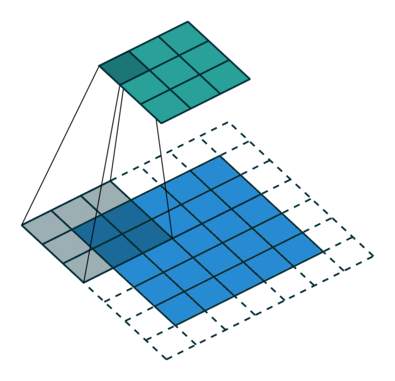
Interactive Convolution Illustration

A basic visual representation of a 2D convolution.

Stride and padding are critical parameters that ECE engineers need to tune when designing CNN architectures, as they directly impact the size of feature maps and the computational load. Stride defines how many pixels the filter moves across the input. A stride of 1 is common, meaning the filter moves one pixel at a time. A larger stride, like 2, causes the filter to skip pixels, effectively downsampling the spatial dimension of the output. This reduces computation but might discard some finer-grained features.

Padding is the practice of adding pixels, usually zeros, around the borders of the input image. This is often done to prevent the spatial dimensions from shrinking too quickly as you apply multiple convolutional layers, and it also ensures that pixels at the edges of the image contribute equally to the features extracted, as they are not “under-sampled.” “Same” padding is popular because it tries to maintain the output dimensions identical to the input.

On this slide, you see the formula for calculating output spatial size. This is a fundamental equation for CNN design. Let’s use the interactive calculator on the left. You can adjust the input size, kernel size, padding, and stride to instantly see the calculated output size. Take the example mentioned in the text: N=32, F=3, P=1, S=1. If you enter these values, you’ll see the output is 32, meaning the input spatial dimension is preserved.

On the right, we have a static diagram of how a convolution operation works, visualizing the sliding window effect. While not interactive, it helps to reinforce the concept for a small input matrix.

Convolutional Operation

Convolutional Operation

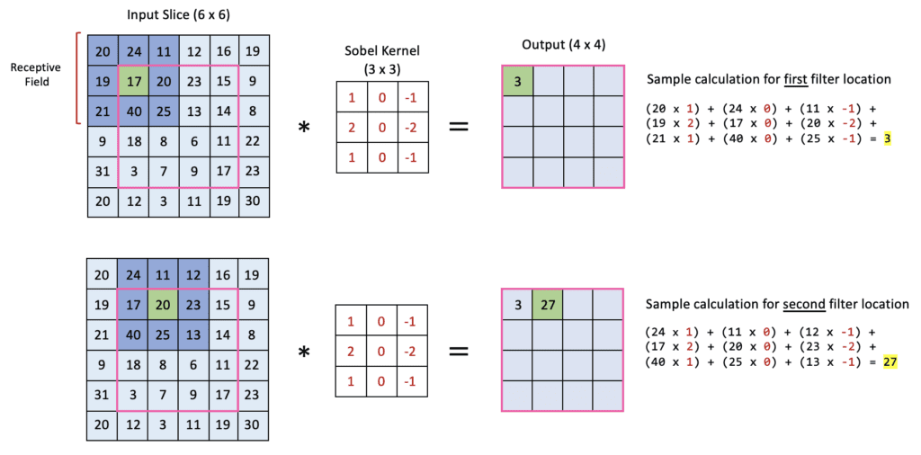
Sobel Kernel: Detecting Vertical Edges

A concrete example of a fixed filter’s operation.

Fixed (Hand-Crafted) Kernel

• Sobel kernel designed to detect vertical edges.
• Comprises positive values on one side, negatives on the other, zeros in middle.
• Acts as a numerical approximation of a derivative in the horizontal direction.
• Output emphasizes sudden intensity changes in the vertical direction.

Note

In CNNs, kernel weights are learned, allowing detection of diverse, complex features, not just predefined edges.

How it Works

Sobel Kernel

To make the convolution concept more tangible, let’s look at a classic example: the Sobel kernel. This is a predefined filter, not a learned one, used to detect vertical edges in an image. As you can see, the kernel has negative values on the left, zeros in the middle, and positive values on the right. When this kernel slides over an image, suppose it encounters a region where pixel values abruptly change from low (dark) to high (bright) from left to right. The negative values in the kernel will amplify the dark pixels, the positive values will amplify the bright pixels, and when summed, will produce a large output value, indicating a strong vertical edge. If there’s no change, the output will be close to zero.

The important distinction here is that while Sobel is fixed, the kernels in CNNs are learned. This means CNNs can discover much more complex and subtle features than simple edges, making them incredibly powerful for diverse vision tasks.

Convolutional Layer Properties

Understanding channels, filters, and trainable parameters.

Filters, Kernels, and Channels

• Filter Depth: Must match input data depth (number of channels).
  • Example: Input (HxWx3) requires filter (fxfrx3).
• Spatial Size (fxfr): Typically 3x3 or 5x5.
• Number of Filters: A design choice, dictates output depth.
  • Multiple filters \(\rightarrow\) Multiple activation maps.
  • Each filter learns a different feature.

Important

A filter is a container for kernels. If input depth is C, a filter has C kernels.

Trainable Parameters

• Number of trainable parameters in a convolutional layer: (kernel_width * kernel_height * input_channels + 1) * num_filters (The +1 is for the bias term per filter.)

Let’s illustrate:

• Input: 224x224x3 (RGB Image)
• Filter: 3x3 spatial size
• Number of Filters: 32

Parameters = (3 * 3 * 3 + 1) * 32 Parameters = (27 + 1) * 32 Parameters = 28 * 32 = 896

• Much fewer than MLPs for large images!

Let’s clarify some terminology around convolutional layers. First, the depth of a filter must always match the depth of the input data it’s convolving with. If your input is a color image with 3 RGB channels, your filter must also have 3 channels or kernels. The spatial size of the filter, like 3x3 or 5x5, is a design decision. Smaller filters are common as they capture local features efficiently. The number of filters in a convolutional layer is another crucial design choice. Each filter specializes in detecting a particular feature. So, if you have 32 filters, that layer will produce 32 activation maps, each highlighting a different learned feature from the input.

A single filter in a convolutional layer is actually a collection of kernels, one for each input channel. So, a filter for a 3-channel input consists of three 2D kernels.

Crucially, let’s look at the trainable parameters. This is where CNNs gain their efficiency. For our example with a 224x224x3 input image, a 3x3 filter, and 32 such filters: Each filter has 3x3x3 = 27 weights (for the 3 input channels) plus 1 bias term. That’s 28 parameters per filter. Multiply this by 32 filters, and you get only 896 trainable parameters for this layer! Compare this to the billions for an MLP. This reduction is a massive advantage from an ECE perspective, making models feasible for embedded systems or real-time applications.

Filters

Convolutional Layer with a Single Filter

Convolutional Layer with Two Filters

Filters Learn to Detect Structure

CNNs Learn Hierarchical Features

From simple edges to complex object parts.

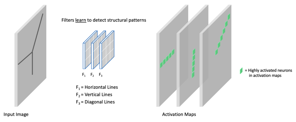
Early Layers: Basic Elements

• Filters in the first layers learn simple, fundamental features.
• Examples: Edges (vertical, horizontal, diagonal), color blobs, textures.
• These are general-purpose features.

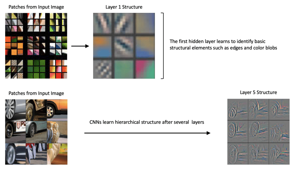
Deeper Layers: Complex Structures

• Filters in deeper layers combine features from previous layers.
• Learn to detect more abstract, composite patterns.
• Examples: Eyes, noses, wheels, ears, specific parts of objects.

Visualizing Feature Learning

Tip

This hierarchical learning is why CNNs are so powerful. They build up complex understanding from simple visual primitives.

CNNs Learn Hierarchical Features

One of the most fascinating aspects of CNNs, and a testament to their deep learning capabilities, is their ability to learn features hierarchically. In the initial layers, the filters tend to detect very basic, low-level features – things like simple edges, lines at different orientations, or blobs of color. These are universal visual primitives.

As the data progresses through subsequent convolutional layers, the filters in these deeper layers don’t look for individual pixels or simple edges anymore. Instead, they combine the basic features detected by the earlier layers to build representations of more complex, abstract patterns. For instance, a filter in a middle layer might learn to detect the pattern of an eye, or a wheel, or a specific texture.

Further still, in very deep layers, these filters can respond to even more complex, semantic parts of an object, like an entire cat’s face or the body of a car. This “part-to-whole” learning or hierarchical feature extraction is what allows CNNs to achieve such incredible performance in tasks like object recognition. The diagram on the right illustrates this progression conceptually.

Pooling Layers: Spatial Dimension Reduction

Summarizing features and reducing computations.

Purpose

• Downsampling: Reduce spatial size of activation maps.
• Reduced Parameters: Decreases input size to subsequent layers.
• Computation Reduction: Faster inference.
• Overfitting Mitigation: Fewer parameters, less memorization.
• Translation Invariance Boost: Small shifts in input yield less change in pooled output.

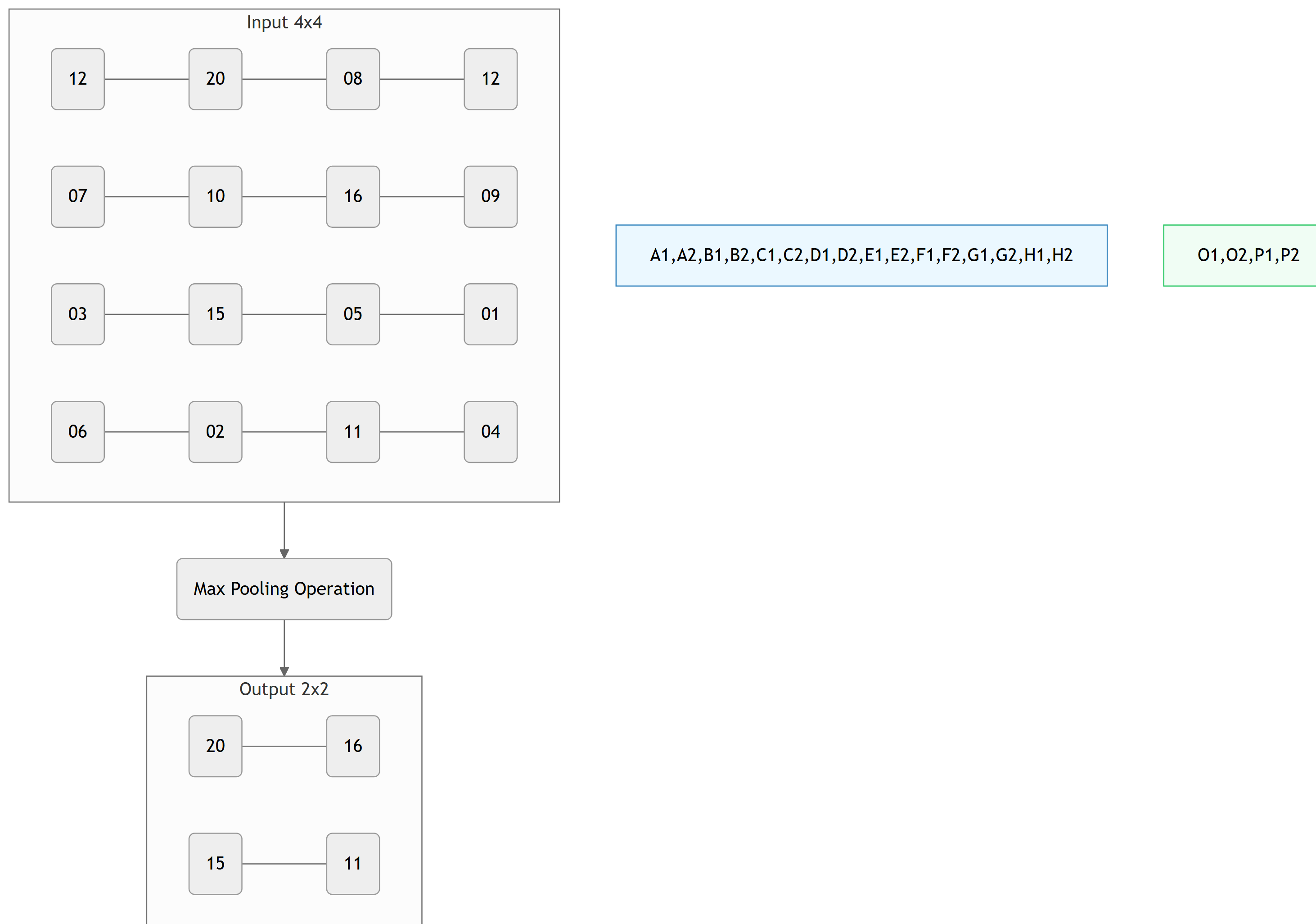
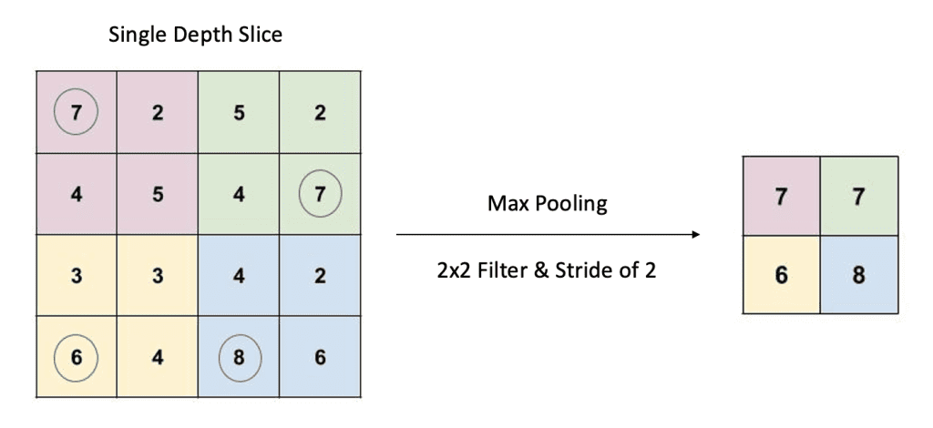
Max Pooling (Most Common)

• A 2D sliding filter (e.g., 2x2).
• Moves across input with a defined stride.
• Outputs the maximum value within the receptive field.
• No trainable parameters in pooling layer itself.

Max Pooling Example

Input 4x4 Activation Map, 2x2 Filter, Stride 2

Note

Pooling layers summarily represent features in a smaller space. Think of it as feature aggregation.

Max Pooling Layers

After extracting features with convolutional layers, we often use pooling layers to reduce the spatial size of the activation maps. This is an important step for several reasons. Primarily, it reduces the number of parameters and computations in the network, making it faster to train and less prone to overfitting. From an ECE perspective, this means more efficient hardware utilization and potentially faster inference times on edge devices. Pooling also provides a form of translation invariance. Even if a feature shifts slightly within its receptive field, the max (or average) value will still likely be captured, leading to a more robust representation.

The most common type is Max Pooling. With a 2x2 filter and a stride of 2, it slides over the input and, for each window, simply picks the maximum value. Look at the example: from a 4x4 input, a 2x2 max pooling with stride 2 yields a 2x2 output. Notice that pooling layers do not have any trainable parameters themselves; they are deterministic operations. This makes them computationally inexpensive.

The Convolutional Block: Building Blocks of Feature Extraction

Combining convolution and pooling.

Typical Structure

• One or more 2D Convolutional Layers:
  • Feature extraction.
  • Followed by activation function (e.g., ReLU).
• Followed by a Pooling Layer:
  • Spatial dimension reduction.
  • Downsize activation maps.

Tip

VGG-16 uses 2-3 convolutional layers before each max pooling layer. Number of filters typically doubles with depth (e.g., 64 \(\rightarrow\) 128 \(\rightarrow\) 256).

Example Block

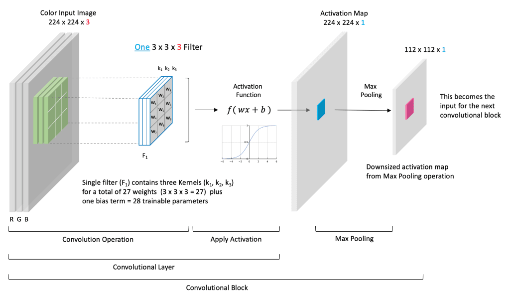
Convolutional Block Detail

A convolutional block is the fundamental repeating unit within the feature extractor of a CNN. It’s where the magic of feature learning and spatial downsampling happens. A typical block involves a sequence of one or more Convolutional layers, each almost always followed by a non-linear activation function like ReLU. After these convolutional layers, a pooling layer, most commonly max pooling, is applied.

The purpose of stacking multiple convolutional layers before pooling is to allow the network to learn increasingly complex features at the same spatial scale before reducing the resolution. Architectures like VGG-16 demonstrate this, using two or three convolutional layers before a max-pooling operation. Also, observe how the number of filters, or output channels, often increases as you go deeper into the network, capturing a richer set of features. This progressive deepening and widening allows for a powerful hierarchical feature representation.

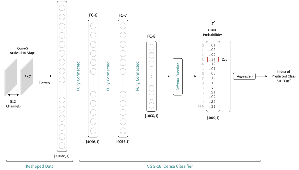
Fully Connected Classifier

Mapping extracted features to class probabilities.

Bridging Features to Decisions

• Connects the high-level features from the feature extractor to dense layers.
• Flattening: Output from the last convolutional block (e.g., 7x7x512) is reshaped into a 1D vector (e.g., 25088 features).
  • Required because dense layers expect 1D input.
• Hidden Dense Layers: Learn complex non-linear combinations of features.
• Output Layer:
  • Number of neurons = Number of classes.
  • Often uses Softmax activation for multi-class probability output ([0,1] range, sums to 1).

Classifier Structure

Note

Flattening doesn’t lose spatial information inherently; it just reorganizes it for the dense layer’s input.

Fully Connected Classifier

Flatenning

Once the feature extractor has done its job of deriving high-level features, the fully connected classifier takes over to make sense of these features and classify the input. The output of the last convolutional block is a 3D tensor, like 7x7x512 in our VGG-16 example. However, traditional fully connected layers expect a 1D vector as input. This is where the flattening step comes in. We simply reshapes this 3D tensor into a long 1D vector. It’s important to note this is just a reorganization of data; no information is lost, and the spatial relationships embedded in the features are still there, implicitly informing the dense layers.

After flattening, the data passes through one or more hidden fully connected layers, which learn intricate non-linear relationships between the extracted features. Finally, the output layer has a number of neurons equal to the number of classes. For multi-class problems, like ImageNet with 1000 classes, a Softmax activation function is typically used. Softmax converts the raw outputs into a probability distribution, where each value is between 0 and 1, and all values sum to 1, indicating the likelihood of the input belonging to each class.

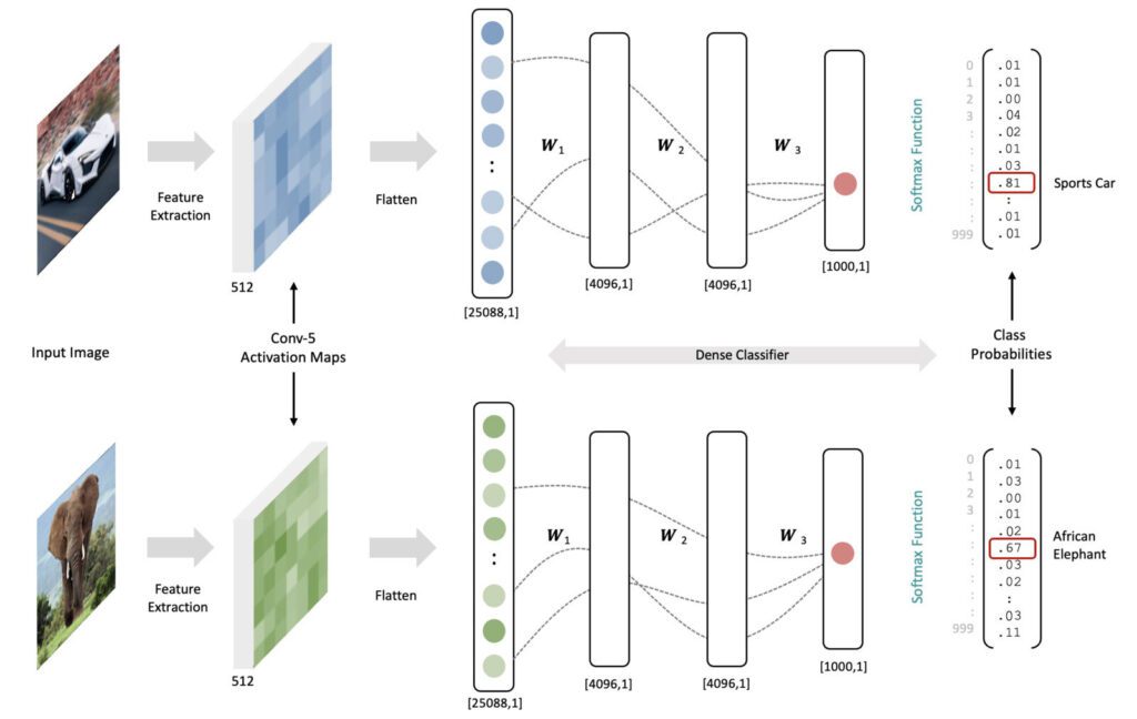
Intuition: How CNNs Map Features to Class Probabilities

Connecting learned features to actionable predictions.

Holistic Understanding of Image Content

• The final activation maps (e.g., 7x7x512) contain rich, meaningful information.
• Each spatial location in these maps retains a relationship to the original input.
• Fully connected layers can process this entire content from the image.

Learned Association

• During training, the weights in the FC layers learn to associate specific feature patterns (from the activation maps) with particular output classes.
• This mapping allows the network to “activate” the correct output neuron based on the combination of features present in the input.

Tip

Minimizing the loss function tunes the weights to effectively map features to class probabilities.

Flow from Features to Prediction

Intuition

It’s easy to get lost in the mathematical details, but the core intuition for why CNNs work in classification is elegant. The feature extractor compresses the vast information of an image into a much smaller, but highly informative, set of high-level features. These features are not just random numbers; they represent semantic components like “has whiskers,” “has round eyes,” or “has four legs” for a cat, for example.

Crucially, the fully connected classifier then takes this rich feature set and learns to associate specific combinations of these features with particular output classes. Through the training process, the billions of connections and weights are adjusted such that if the network “sees” features indicative of a cat, the neuron corresponding to “cat” in the output layer will strongly activate.

The process of minimizing a loss function during training guides this learning, forcing the network to adjust its weights so that it correctly maps input images to their true labels. This entire pipeline, from hierarchical feature extraction to learned classification, is why CNNs are so effective. For ECE this translates to robust object detection in autonomous vehicles, or reliable anomaly detection in medical images.

Additional Topics in CNNs

Enhancing training and performance.

1. Dropout

• Purpose: Regularization technique to prevent overfitting.
• Mechanism: Randomly sets a fraction of neurons’ activations to zero during training.
• Benefit: Forces network to learn more robust features, less reliant on specific neurons.

2. Batch Normalization

• Purpose: Stabilize and accelerate network training.
• Mechanism: Normalizes layer inputs by subtracting batch mean and dividing by batch standard deviation.
• Benefit: Reduces “internal covariate shift,” improves gradient flow, allows higher learning rates.

3. 3D Convolution

• Extension of 2D Convolution: Kernel shifts across three axes (height, width, AND depth/time).
• Applications:
  • Medical Imaging: Analyzing volumetric data (e.g., MRI, CT scans).
  • Video Processing: Capturing spatio-temporal features across frames.
• Benefit: Captures spatial relationships and temporal/depth relationships.

Spatio-temporal Feature Extraction

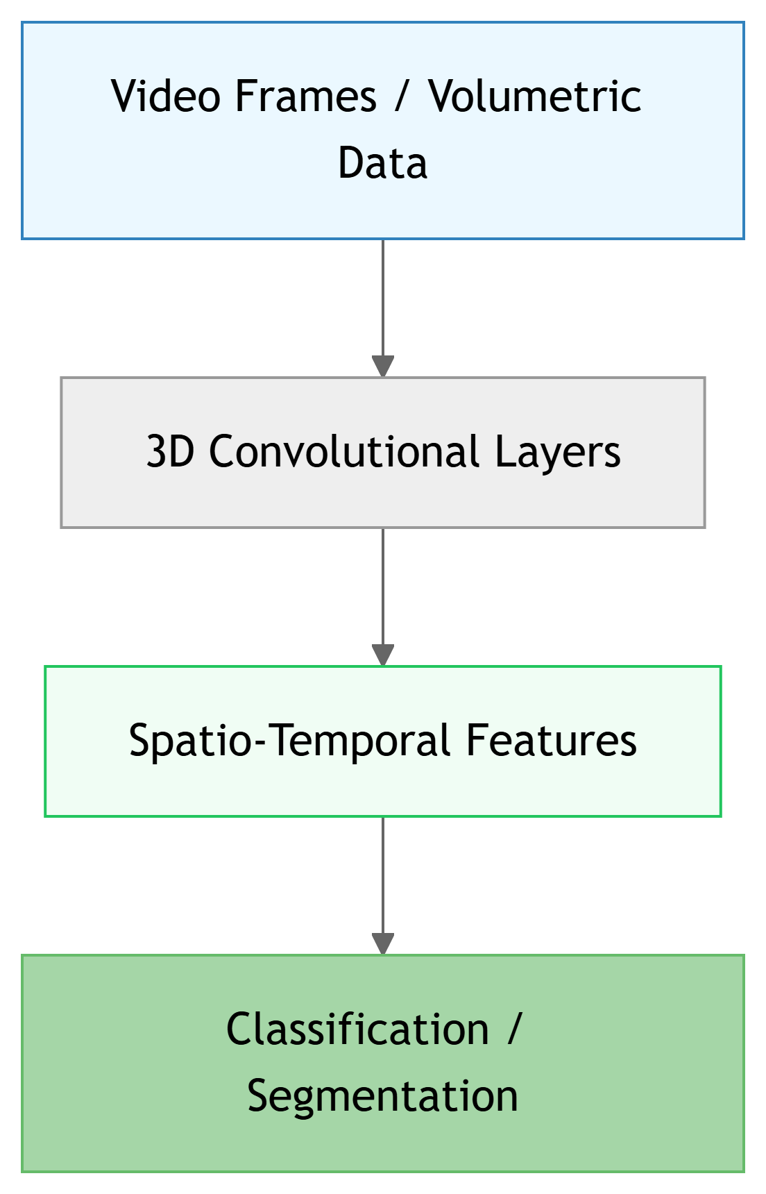
Note

Crucial for dynamic signals and volumetric data in ECE applications.

Beyond the core architecture, ECE engineers often employ several techniques to improve CNN training and performance. Dropout is a powerful regularization technique. During training, it randomly “drops out” or deactivates a percentage of neurons in a layer. This prevents complex co-adaptations between neurons and forces the network to learn more redundant and robust feature representations, mitigating overfitting.

Batch Normalization is another critical technique. It normalizes the inputs to layers by adjusting them to have zero mean and unit variance for each mini-batch during training. This stabilizes the learning process, prevents exploding or vanishing gradients, and allows for faster training with potentially higher learning rates.

Finally, 3D Convolution extends the concept of 2D convolution to handle volumetric data or sequential data like videos. Instead of a 2D filter, we use a 3D filter that slides not just across height and width, but also across depth (for volumetric data) or time (for video frames). This allows the network to learn spatio-temporal features, which is incredibly useful in ECE domains like medical image analysis for 3D scans, or video surveillance and action recognition.

Summary of Key Points

Consolidating our understanding of CNNs.

• CNNs vs. MLPs: CNNs overcome MLP limitations for images (translation invariance, parameter efficiency).
• Architecture: Comprise a Feature Extractor (Convolutional Blocks) and a Classifier (Fully Connected Layers).
• Convolutional Layers:
  • Use learned filters/kernels to extract features.
  • Parameter sharing crucial for efficiency.
  • \[ O = \left\lfloor \frac{n - f + 2p}{s} \right\rfloor + 1 \] governs output size.
• Pooling Layers:
  • Downsample activation maps (e.g., Max Pooling).
  • Reduce parameters, computation, and mitigate overfitting.

• Hierarchical Features: CNNs learn from simple edges to complex object parts.
• Fully Connected Classifier:
  • Flattens features and maps them to class probabilities via dense layers + Softmax.
• Enhancements:
  • Dropout: Regularization to prevent overfitting.
  • Batch Normalization: Stabilizes and accelerates training.
  • 3D Convolution: For spatio-temporal or volumetric data.

Important

CNNs are the backbone of modern computer vision, driving innovation in diverse ECE applications.

To wrap up, let’s quickly review the main concepts we covered today. We started by understanding why CNNs were developed – to address the limitations of traditional MLPs when dealing with high-dimensional image data, particularly concerning translation invariance and the explosion of trainable parameters. We then explored the two main components of a CNN: the feature extractor, built from convolutional blocks, and the fully connected classifier. We deep-dived into convolutional layers, understanding how learned filters extract features through operations influenced by stride and padding, and how the output feature map size is calculated. Remember the formula! We looked at pooling layers, especially max pooling, and their role in downsampling, reducing complexity, and helping to prevent overfitting. A core strength of CNNs is their ability to learn hierarchical features, starting with basic edges and building up to complex patterns. The fully connected classifier then takes these rich features, flattens them, and maps them to final class probabilities using dense layers and Softmax. Finally, we touched upon practical techniques like Dropout and Batch Normalization for improving training, and the concept of 3D convolution for advanced applications involving volumetric or video data. All these elements together make CNNs indispensable tools for ECE professionals working in areas like autonomous systems, medical diagnostics, robotics, and more.