Machine-Learning-03

Tensorflow, Keras, Deep Learning

Imron Rosyadi

Introduction to CNNs

Bridging Theory and ECE Applications

What is a CNN?

• A type of neural network specialized in processing data with a grid-like topology.
• Primarily used for image recognition, computer vision, and signal processing.
• Inspired by the human visual cortex.

Filtering an image with two successive filters, each made of 4x4x3=48 learnable weights.

CNNs are a cornerstone of modern AI, especially for tasks involving spatial data. For ECE students, it’s not just about theoretical understanding but also about their practical implementation in hardware and software for real-world applications. This introductory slide sets the stage for diving into the core mechanisms.

Core Concept: The Convolution Operation

A Localized Filtering Approach

Localized Receptive Fields

• Unlike dense layers where each neuron sees the entire input, a CNN neuron processes only a small, local region of the input (its receptive field).
• This significantly reduces the number of learnable parameters.

Weight Sharing (Filtered Operations)

• The same set of weights (a filter or kernel) is applied across the entire image.
• This operation is known as convolution.
  • It acts like a digital filter, detecting specific features (edges, textures, patterns).

Note

This operation is analogous to applying FIR/IIR filters in digital signal processing, but here the filter coefficients are learned.

Core Concept: The Convolution Operation

A Localized Filtering Approach

Analogy: Each filter creates a “feature map” or “channel” highlighting specific patterns.

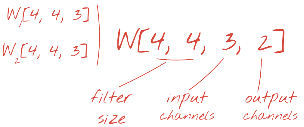
Why Multiple Filters/Channels?

• A single filter might detect one type of feature (e.g., horizontal edges).
• To detect a variety of features, we use multiple filters.
• Each filter produces a separate output channel or feature map.
• These multiple channels are stacked to form a new “data cube”.

Visualizing the Convolution Operation

An Interactive Example

Input: A simple 2D grid representing an image or signal.

Kernel: A smaller 2D filter that slides over the input.

Operation: At each position, the kernel’s values are multiplied element-wise by the corresponding input values within its receptive field, and the products are summed to form a single output pixel.

Key Parameters:

• Kernel Size: Dimensions of the filter (e.g., 3x3, 5x5).
• Stride: Number of pixels the filter shifts at each step.
• Padding: Adding zeros to the input edges to preserve spatial dimensions.

Visualizing the Convolution Operation

An Interactive Example

viewof input_size = Inputs.range([3, 10], {value: 5, step: 1, label: "Input Size (N x N)"});
viewof kernel_size = Inputs.range([1, 3], {value: 3, step: 2, label: "Kernel Size (K x K)"});

This interactive slide allows students to dynamically adjust input and kernel sizes to see how the convolution operation changes. It visually demonstrates the concept of a sliding window. Emphasize that in actual CNNs, the kernel values are learned through backpropagation, not randomly assigned. This interactivity helps bridge the abstract concept with a concrete visual.

Building Blocks of a CNN

Layer by Layer

Convolutional Layer (Conv2D)

• Applies a set of learnable filters to the input image / feature maps.
• Generates new feature maps that highlight specific patterns.
• Parameters: filters, kernel_size, strides, padding, activation.

Activation Function (ReLU)

• Introduces non-linearity to the model.
• ReLU (Rectified Linear Unit) is popular due to its computational efficiency.
  • \(f(x) = \max(0, x)\)

Pooling Layer (Max Pooling, GlobalAveragePooling2D)

• Reduces the spatial dimensions of the feature maps.
• Decreases computation and helps control overfitting.
• Max Pooling: Takes the maximum value from each patch.
• GlobalAveragePooling2D: Averages entire feature maps, often used before the final classification.

Building Blocks of a CNN

Layer by Layer

Example Keras Model Snippet:

model = tf.keras.Sequential([
    tf.keras.layers.Reshape(input_shape=(28*28,), target_shape=(28, 28, 1)),
    tf.keras.layers.Conv2D(kernel_size=3, filters=12, activation='relu'),
    tf.keras.layers.Conv2D(kernel_size=6, filters=24, strides=2, activation='relu'),
    tf.keras.layers.Conv2D(kernel_size=6, filters=32, strides=2, activation='relu'),
    tf.keras.layers.Flatten(), # or GlobalAveragePooling2D()
    tf.keras.layers.Dense(10, activation='softmax')
])

Dense Layer (Dense)

• A fully connected layer, typically at the end of the network.
• Used for classification, after the spatial features have been extracted and flattened.

Flatten Layer (Flatten)

• Converts the multi-dimensional output of convolutional/pooling layers into a 1D vector.
• Prepares the data for input to a dense layer.

Architectural View of a CNN

Data Cubes in Motion

Data Transformation:

• A CNN can be visualized as transforming “cubes” of data.
• Each operation (convolution, pooling) manipulates the dimensions of these cubes.

Input Layer:

• Starts with an input image (e.g., 28x28x1 for grayscale MNIST, 224x224x3 for RGB images).

Intermediate Layers:

• Convolutional layers increase the number of channels (filters) while possibly reducing spatial dimensions (if strides > 1).
• Pooling layers reduce spatial dimensions, preserving the number of channels.

Output Layer:

• Typically, a Flatten or GlobalAveragePooling2D layer converts the cube into a vector.
• Followed by a Dense layer with a softmax activation for classification probabilities.

Important

The precise management of spatial dimensions (height, width) and channels is a key ECE consideration for memory and computational efficiency.

This diagram visually reinforces the concept of data flowing as “cubes” through different layers, changing their dimensions. Explain how each layer type manipulates the height, width, and channel dimensions. For ECE, also consider how these dimension changes impact memory bandwidth and computational load on custom hardware accelerators.

Strided Convolutions & Max Pooling

Downsampling Strategies

Purpose of Downsampling:

• Reduce computational load: Fewer pixels to process in subsequent layers.
• Extract more abstract features: Larger receptive fields for higher-level features.
• Increase robustness: Make the network less sensitive to small shifts or distortions in the input.

1. Strided Convolution:

• The convolution filter moves by stride pixels at each step (e.g., stride=2).
• Directly reduces the output feature map size.
• Example: tf.keras.layers.Conv2D(..., strides=2, ...)

2. Max Pooling:

• A non-parametric operation.
• Slides a window (e.g., 2x2) across the feature map.
• Outputs the maximum value within that window.
• Commonly used with pool_size = strides (e.g., 2x2 window with stride 2).
• Example: tf.keras.layers.MaxPooling2D(pool_size=(2, 2), strides=(2, 2))

Strided Convolutions & Max Pooling

Downsampling Strategies

Strided convolutions or max pooling reduce spatial dimensions.

Note

In ECE, choice between strided convolution and pooling impacts hardware architecture. Strided convo uses multiply-accumulate units. Max pooling requires comparators and a maximum selector.

Comparison:

• Strided Conv: Learns how to downsample, can adapt filters for optimal feature reduction.
• Max Pooling: Simpler, fixed operation; preserves only the most salient features. Reduces overfitting by taking only the maximum.

The Final Layer: Classification Head

Connecting Features to Decisions

Goal: Transform the extracted features into class probabilities.

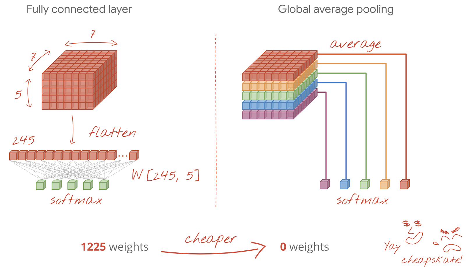
Option 1: Flatten and Dense Layers

1. Flatten: Converts the 3D feature cube into a 1D vector.
   • tf.keras.layers.Flatten()
2. Dense Layer(s): One or more fully connected layers.
   • Can be computationally expensive.
   • High number of weights, especially for large feature maps.
3. Softmax Activation: Last dense layer outputs probabilities for each class.

Warning

A large Flatten output connected to a Dense layer can lead to a parameter explosion, a major concern for memory and computation in embedded ECE systems.

Option 2: Global Average Pooling (GAP) and Dense/Softmax

1. GlobalAveragePooling2D:
   • Averages each feature map across its spatial dimensions (height x width).
   • Converts a [H x W x C] cube into a [C] vector.
   • Example: tf.keras.layers.GlobalAveragePooling2D()
2. Dense Layer (optional) / Softmax:
   • Often, this is fed directly into a final Dense layer with softmax.
   • 0 weights if directly connected to output softmax layer (no intermediate Dense layer).
   • Significantly reduces parameters and helps prevent overfitting.

Tip

For ECE applications, especially on resource-constrained devices, GlobalAveragePooling2D is often preferred for its parameter efficiency.

The Final Layer: Classification Head

Connecting Features to Decisions

Two options for the final layer.

Conclusion

Key Takeaways for ECE

Recap of CNN Fundamentals:

• Localized Receptive Fields: Neurons respond to small regions.
• Weight Sharing: Filters slide across the input, making CNNs efficient.
• Feature Hierarchy: Layers progressively learn more complex features.
• Downsampling: Strided convolutions and pooling reduce data dimensions, manage computation.
• Classification Head: Flatten + Dense or GlobalAveragePooling2D for final prediction.

Conclusion

Key Takeaways for ECE

Relevance for Electrical and Computer Engineers:

• Hardware Acceleration: Designing custom chips (ASICs, FPGAs) for efficient CNN inference.
• Embedded AI: Deploying CNNs on low-power, edge devices (e.g., IoT, drones, automotive ECUs).
• Sensor Fusion: Processing data from multiple ECE sensors (cameras, LiDAR, radar) using CNNs.
• Real-time Processing: Optimizing CNN architectures and implementations for latency-critical applications.
• Resource Optimization: Balancing accuracy with computational cost, power consumption, and memory footprint.

Reinforce the practical implications of CNN knowledge. Emphasize that ECE professionals don’t just use these models, they build the underlying hardware and software tools that make them possible, and they face unique challenges related to resource constraints and real-time performance.

Regularization: Dropout

Mitigating Overfitting in Machine Learning Models

Understanding Overfitting

A Critical Challenge in ML

What is Overfitting?

• A model that performs exceptionally well on the training data but poorly on unseen data (validation/test data).
• The model essentially “memorizes” the training examples, including noise and specific patterns, rather than learning generalizable features.

Signs of Overfitting:

1. Training Loss Decreases: Continues to go down during training.
2. Validation Loss Increases: Starts to rise after an initial decrease, indicating the model is losing generalization ability.
3. High Training Accuracy, Low Validation Accuracy: A significant gap between performance on seen and unseen data.

Causes of Overfitting:

• Model Complexity: Too many parameters or layers relative to data.
• Insufficient Data: Not enough training examples to learn general patterns.
• Noisy Data: The model learns to fit the noise in the training set.

Warning

For ECE applications, overfitting can lead to unreliable system performance in real-world scenarios, which is unacceptable for safety-critical systems like autonomous vehicles or medical devices.

Understanding Overfitting

A Critical Challenge in ML

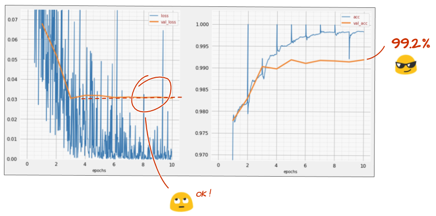
Validation loss flattening and training loss decreasing, a positive sign with dropout.

Introduction to Dropout

A Simple Yet Powerful Regularization Technique

What is Dropout?

• A regularization technique introduced by Hinton et al. in 2012.
• Randomly sets a fraction of neuron outputs to zero at each training step.
• “Dropping out” neurons means they temporarily do not contribute to the forward pass and do not participate in backpropagation.

Analogy:

• Imagine a team where, for each task, a random subset of members is absent. The remaining members must learn to perform their roles more robustly without relying on any single individual.

Introduction to Dropout

A Simple Yet Powerful Regularization Technique

How it Works (Training Phase):

• A dropout rate (e.g., 0.2 to 0.5) specifies the probability of a neuron being dropped.
• Each neuron has its state (active/inactive) sampled independently.
• The weights of the remaining active neurons are scaled up by 1 / (1 - dropout_rate) to maintain the same expected sum of outputs.

Inference/Testing Phase:

• All neurons are active and contribute to the output.
• Their weights are not scaled (or equivalently, they are pre-scaled by the dropout rate during training).

Explain that dropout is like training an ensemble of neural networks, where each epoch a different “thinned” network is trained. This forces the network to learn more robust features that are not reliant on specific co-adaptations of neurons. Emphasize the difference between training (random drops and scaling) and inference (all neurons active, no scaling).

Dropout in Keras

Implementation and Placement

Adding Dropout Layers:

• In Keras, dropout is implemented as a layer: tf.keras.layers.Dropout(rate).
• The rate is the fraction of inputs to drop (e.g., 0.2 for 20%).

Typical Placement:

• Often applied after activation functions (or after convolutional and pooling layers, before Flatten or Dense).
• Commonly used after convolutional blocks and before fully connected (dense) layers to prevent overfitting on extracted features.

Example Keras Model with Dropout:

model = tf.keras.Sequential([
    tf.keras.layers.Reshape(input_shape=(28*28,), target_shape=(28, 28, 1)),
    tf.keras.layers.Conv2D(kernel_size=3, filters=12, activation='relu'),
    tf.keras.layers.MaxPooling2D(pool_size=(2,2), strides=(2,2)), # Added pooling
    tf.keras.layers.Dropout(0.25), # Dropout after pooling
    tf.keras.layers.Conv2D(kernel_size=6, filters=24, strides=1, activation='relu'),
    tf.keras.layers.MaxPooling2D(pool_size=(2,2), strides=(2,2)), # Another pooling
    tf.keras.layers.Dropout(0.25), # Dropout after second pooling
    tf.keras.layers.Flatten(),
    tf.keras.layers.Dense(128, activation='relu'), # Intermediate Dense layer
    tf.keras.layers.Dropout(0.5), # High dropout for dense layers
    tf.keras.layers.Dense(10, activation='softmax')
])

Dropout in Keras

Implementation and Placement

Practical Considerations:

• Dropout Rate:
  • Usually between 0.2 and 0.5. Needs tuning.
  • Higher rates for larger models or smaller datasets.
• Placement: Experiment with placement.
  • Often effective before dense layers due to their high parameter count.
  • Can be used after convolutional layers too.
• Training Time: Dropout can sometimes increase training time as the network needs more iterations to converge.

Tip

In ECE, understanding dropout’s impact on model robustness is critical. A robust model performs reliably even with minor input variations, which is vital for real-world environmental noise or sensor inaccuracies.

Dropout in Keras

Dropout Effect on Training

This Python code block does not execute a full training loop to demonstrate dropout, but illustrates how the dropout layer works by modifying input tensors.

#| max-lines: 10
import tensorflow as tf
import numpy as np

# Create a sample input tensor (e.g., output from a previous layer)
input_tensor = tf.constant(np.arange(1, 11, dtype=np.float32).reshape(1, 10))
print("Original Input Tensor:")
print(input_tensor.numpy())

# Create a Dropout layer with a rate of 0.5
dropout_layer = tf.keras.layers.Dropout(rate=0.5)

# Simulate training mode (where dropout is active)
# The is_training=True argument is crucial for Dropout to be active
dropped_output = dropout_layer(input_tensor, training=True)
print("\nOutput with Dropout (training=True):")
print(dropped_output.numpy())

# Simulate inference mode (where dropout is inactive, and scaling is applied - though handled internally)
regular_output = dropout_layer(input_tensor, training=False)
print("\nOutput without Dropout (training=False - all values present, no explicit scaling shown here as it's for weights):")
print(regular_output.numpy())

The interactive example shows how Dropout literally sets some values to zero in training. Emphasize that in inference, no values are dropped, and all neurons contribute. The scaling factor applied during training (or to weights during inference, depending on implementation) ensures the expected output magnitude remains consistent.

When Dropout Helps (and When It Doesn’t)

Diagnosing Overfitting

When Dropout is Effective:

• Overfitting is the primary problem: When validation loss starts increasing while training loss continues to decrease.
• Complex Models: Helps prevent co-adaptation of neurons in deep architectures.
• Sufficiently Large Datasets: Dropout works best when the model has enough data to learn diverse features across different “sub-networks.”

When Dropout Might Not Help (or Even Hurt):

• Underfitting: If the model is too simple or data is too scarce, dropout can make it even harder for the model to learn.
• Wrong Architecture: If the model itself is fundamentally unsuited for the task (e.g., fully connected layers for image data without convolutions).
  • In such cases, dropout cannot compensate for a poor architectural design.
• Too High Dropout Rate: Can lead to underfitting if too many neurons are dropped, effectively simplifying the network too much.

When Dropout Helps (and When It Doesn’t)

Diagnosing Overfitting

Analyzing Loss Curves:

• Training loss decreasing, Validation loss increasing: Classic sign of overfitting \(\rightarrow\) Use Dropout.
• Both training and validation loss decreasing but high: Underfitting or insufficient capacity \(\rightarrow\) Adjust architecture, add layers, remove dropout.
• Both training and validation loss erratic: Learning rate too high, batch size too small, or bad initialization \(\rightarrow\) Adjust hyperparameters.

Note

For ECE systems, debugging model performance requires a systematic approach. Distinguishing between architectural issues, data limitations, and overfitting is key to efficient resource allocation in hardware design and algorithm tuning.

Beyond Dropout: Other regularization techniques include L1/L2 regularization, data augmentation, batch normalization, and early stopping.

Conclusion

Dropout Summary & ECE Relevance

Key Learnings about Dropout:

• Mechanism: Randomly deactivates neurons during training to prevent co-adaptation.
• Goal: Mitigates overfitting, leading to better generalization on unseen data.
• Implementation: Simple Keras Dropout layer.
• Diagnosis: Effective when validation loss deviates upwards from training loss.

Conclusion

Dropout Summary & ECE Relevance

ECE Relevance:

• Robustness: Dropout improves model robustness, crucial for deployment in noisy or varying real-world environments (e.g., sensor data processing).
• Deployment Reliability: Reduces the chance of models failing on edge cases not perfectly represented in the training data, enhancing system reliability.
• Model Selection: ECE engineers need to select appropriate regularization techniques to optimize the trade-off between model accuracy, complexity, and deployment constraints (memory, power).
• Debugging: Understanding loss curves and the role of regularization is vital for efficient troubleshooting and performance tuning of hardware-accelerated ML systems.

Conclude by reiterating the direct benefits of dropout for ECE students: not just better theoretical understanding, but practical tools for building more reliable and robust intelligent systems. Emphasize that regularization is a critical skill for any ECE professional working with AI/ML.

Batch Normalization

Stabilizing and Accelerating Neural Network Training

The Challenge of Internal Covariate Shift

Why Normalization is Needed in Deep Networks

Internal Covariate Shift (ICS):

• During neural network training, the distribution of inputs to hidden layers changes as the parameters of the preceding layers change.
• This continuous shift means that a layer constantly has to adapt to a new input distribution.
• Analogy: Imagine trying to learn to ride a bike where the ground underneath is constantly shifting.

Problems Caused by ICS:

• Slower Training: Requires lower learning rates and careful initialization.
• Vanishing/Exploding Gradients: Can make activations too small or too large.
• Difficulty in Optimization: Makes it harder for the optimizer to find good weights.
• Reduced Generalization: Can negatively impact model performance.

Warning

Understanding and mitigating ICS is crucial for ECE, especially in designing custom hardware for deep learning, as it impacts convergence speed and resource utilization.

The Challenge of Internal Covariate Shift

Why Normalization is Needed in Deep Networks

Conceptual representation of the impact of Batch Normalization, allowing for smoother training curves.

How Batch Normalization Addresses ICS:

• Standardizes the inputs to hidden layers.
• It normalizes the activations of each previous layer at each mini-batch, making the distribution more stable.
• For each feature/channel across the mini-batch, it computes the mean and variance, then normalizes the data to have zero mean and unit variance.

What is Batch Normalization?

The Mechanism

Per-Batch, Per-Feature Normalization:

For each mini-batch during training, and for each feature (or channel in CNNs) independently:

1. Calculate Mean (\(\mu_B\)): Compute the mean of the activations for that feature across all samples in the mini-batch.
2. Calculate Variance (\(\sigma_B^2\)): Compute the variance of the activations for that feature across all samples in the mini-batch.
3. Normalize: Scale the activations to have zero mean and unit variance. \[ \hat{x}_i = \frac{x_i - \mu_B}{\sqrt{\sigma_B^2 + \epsilon}} \] (\(\epsilon\) is a small constant for numerical stability)
4. Scale and Shift: Apply learnable parameters \(\gamma\) (scale) and \(\beta\) (shift) to restore representation power. \[ y_i = \gamma \hat{x}_i + \beta \]
   • \(\gamma\) and \(\beta\) allow the network to learn optimal mean/variance for each layer, not just forcing it to be 0 and 1.
   • These are trained parameters, just like weights and biases.

What is Batch Normalization?

The Mechanism

Training vs. Inference:

• Training: Mean and variance are calculated per mini-batch.
• Inference: Moving averages of mean and variance (collected during training) are used.
  • Ensures deterministic output for a single input, as batch statistics are unavailable.

Detail the four steps of Batch Norm. Emphasize that \(\gamma\) and \(\beta\) are learnable parameters, making Batch Norm a flexible transformation, not just a rigid standardization. Clarify the different behavior during training (batch statistics) and inference (running averages). This distinction is critical for ECE in deployment.

Benefits of Batch Normalization

Why it’s a Game Changer

1. Faster Training (Higher Learning Rates):
   • Stabilizes gradients, allowing for much higher learning rates without risk of divergence.
   • This significantly reduces training time.
2. Reduces Impact of Initialization:
   • Less sensitive to initial weights.
   • The normalization process acts as a buffer against poor initial conditions.
3. Regularization Effect:
   • Adds a slight amount of noise to the network’s activations, much like dropout.
   • Can sometimes reduce or negate the need for dropout, as seen in the text.
4. Improved Gradient Flow:
   • Prevents vanishing/exploding gradients in very deep networks by keeping activation distributions stable.

Tip

For ECE, faster training means shorter design cycles and more iterations for experimentation, while improved stability leads to more robust and deployable ML models.

Benefits of Batch Normalization

Why it’s a Game Changer

Impact on Training Curves:

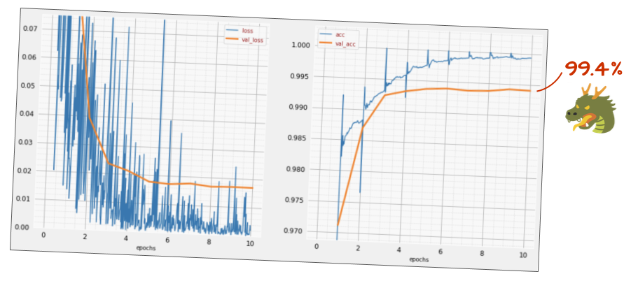
Batch Norm often leads to smoother, faster convergence to higher accuracy.

Practical Rules of Thumb from the Reference:

• Batch Norm helps neural networks converge and usually allows you to train faster.
• Batch Norm is a regularizer. You can usually decrease the amount of dropout you use, or even not use dropout at all.

Implementing Batch Normalization in Keras

Practical Integration

Keras Layer:

• Implemented as tf.keras.layers.BatchNormalization().

Placement:

• Typically placed after a convolutional or dense layer and before its activation function.
• Why use_bias=False? The beta parameter in Batch Norm effectively acts as a bias term, so the biases from the preceding Conv2D or Dense layer are redundant.
• Why scale=False for ReLU? For ReLU, scale=False can sometimes be used because ReLU sets negative values to zero, and the learned \(\gamma\) parameter might not be strictly necessary for scaling. However, scale=True (default) is generally fine and allowing \(\gamma\) to be learned provides more flexibility.

Example Keras Snippet:

# Original approach with activation in the layer
# tf.keras.layers.Conv2D(kernel_size=3, filters=12, activation='relu')

# With Batch Normalization:
model = tf.keras.Sequential([
    tf.keras.layers.Conv2D(kernel_size=3, filters=12, use_bias=False), # No bias
    tf.keras.layers.BatchNormalization(scale=True), # Default scale=True
    tf.keras.layers.Activation('relu'), # Activation after Batch Norm
  
    tf.keras.layers.Conv2D(kernel_size=6, filters=24, strides=2, use_bias=False),
    tf.keras.layers.BatchNormalization(scale=True),
    tf.keras.layers.Activation('relu'),
  
    tf.keras.layers.Flatten(),
    tf.keras.layers.Dense(128, use_bias=False),
    tf.keras.layers.BatchNormalization(scale=True),
    tf.keras.layers.Activation('relu'),
    tf.keras.layers.Dense(10, activation='softmax') # No Batch Norm here
])

Implementing Batch Normalization in Keras

Practical Integration

Interactive Example: Batch Norm Effect on Activation Distribution

viewof mean_val = Inputs.range([-2, 2], {value: 0.5, step: 0.1, label: "Input Mean"});
viewof std_val = Inputs.range([0.1, 3], {value: 1.5, step: 0.1, label: "Input Std Dev"});

The interactive demo clearly shows how Batch Normalization transforms an arbitrary input distribution to one with approximately zero mean and unit variance. This visual “stabilization” helps students intuitively grasp the core idea of reducing internal covariate shift. Explain that the gamma and beta parameters (set to 1 and 0 here for simplicity) allow the network to ‘undo’ this if needed, but the normalization acts as a helpful processing step.

Conclusion

Batch Normalization’s Impact on Modern ML

Key Takeaways on Batch Normalization:

• Addresses Internal Covariate Shift: Stabilizes the input distribution to layers.
• Accelerates Training: Allows higher learning rates and faster convergence.
• Acts as a Regularizer: Reduces the need for dropout.
• Improves Gradient Flow: Aids optimization in deep networks.
• Implementation: tf.keras.layers.BatchNormalization() typically placed between a layer and its activation, with use_bias=False in the preceding layer.

Conclusion

Batch Normalization’s Impact on Modern ML

Significance for ECE Professionals:

• Hardware Efficiency: Designing efficient hardware accelerators for Batch Normalization (e.g., dedicated arithmetic units for mean/variance, fixed-point implementations).
• Embedded Systems: Crucial for deploying deep models on resource-constrained devices, as faster training means quicker model updates and fewer training epochs.
• Power Optimization: Faster convergence contributes to less power consumption during training.
• Robust Model Design: Leads to more stable and robust models, essential for mission-critical ECE applications in real-world deployments.
• State-of-the-Art Models: Batch Normalization is a fundamental component of almost all modern, high-performing deep learning architectures.

Conclude with a strong emphasis on why Batch Normalization is indispensable for ECE students. It’s not just an algorithmic trick but a critical component influencing hardware design, deployment strategies, and overall system performance in AI-driven ECE applications. Highlight its role in enabling the development of deeper, more complex, and more effective neural networks.