Machine-Learning-03

Tensorflow, Keras, Deep Learning

Imron Rosyadi

Overview: Recognizing Handwritten Digits

Today, we’ll dive into building a neural network to recognize handwritten digits.

We’ll achieve ~99% accuracy using fewer than 100 lines of Python/Keras code.

This is a classic problem in Machine Learning, often tackled with the MNIST dataset.

Welcome to this lecture on Deep Learning for ECE! Today, we’re going to tackle a fascinating problem: teaching a computer to recognize handwritten digits. This isn’t just a theoretical exercise; it has real-world applications in areas like postal code recognition, check processing, and even automated data entry.

We’ll be using one of the most famous datasets in machine learning, MNIST, which consists of tens of thousands of handwritten digits. Our goal is ambitious: to achieve around 99% accuracy. And the best part? We’ll do it with remarkably concise code using Python’s TensorFlow and Keras libraries. This means focusing on the concepts and building blocks rather than getting bogged down in low-level details.

What You’ll Learn

This session will cover key concepts and practical techniques:

• What a neural network is and how it learns.
• Building basic 1-layer neural networks with tf.keras.
• Adding more layers for improved performance.
• Implementing learning rate schedules.
• Introduction to Convolutional Neural Networks (CNNs).
• Regularization techniques: Dropout and Batch Normalization.
• Understanding and mitigating overfitting.

Here’s a roadmap of what we’ll cover. We’ll start with the fundamentals of neural networks, then progressively build more complex models. We’ll explore techniques to optimize training, such as learning rate schedules, and introduce you to Convolutional Neural Networks, which are particularly powerful for image data like the MNIST digits. We’ll also discuss critical techniques like dropout and batch normalization to ensure our models are robust, and we’ll address the common pitfall of overfitting.

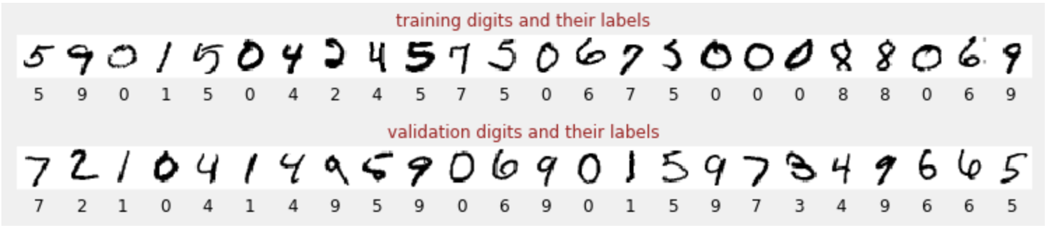
Understanding the Training Data: MNIST

The MNIST dataset contains 60,000 labeled images of handwritten digits (0-9).

Each image is associated with its correct numerical label.

This “labeled dataset” is crucial for training.

Our neural network learns to classify these images into 10 classes (0 through 9).

Example MNIST Digits:

The core of any supervised machine learning task is the data, and for image classification, especially with neural networks, we need labeled data. The MNIST dataset is a classic example. It comprises 60,000 images, each a 28x28 pixel grayscale representation of a handwritten digit, and crucially, each image comes with a label indicating the actual digit it represents. For instance, an image of a handwritten ‘5’ is accompanied by the label ‘5’. This labeled data is what allows our neural network to learn by example.

Training vs. Validation Datasets

How do we assess our model’s “real-world” performance?

• Training Dataset: Used to update the model’s internal parameters. The model sees this data multiple times.
• Validation Dataset: A separate, unseen labeled dataset to evaluate performance and prevent cheating. It reflects how well the model generalizes to new data.

Important

Using “unseen” data for validation is fundamental for robust model evaluation.

It’s vital to know if our trained neural network can generalize its knowledge to new, unseen examples. If we only tested it on the data it was trained on, it would likely perform exceptionally well, but that wouldn’t tell us if it’s truly learned the underlying patterns or just memorized the training examples. This is where the distinction between training and validation datasets comes in.

The training dataset is like the practice problems you do to learn a subject. The model sees these examples, adjusts its internal parameters, and tries to get better.

The validation dataset is like a surprise pop quiz. The model has never seen these examples before. Its performance on this dataset gives us an unbiased estimate of how well it will perform on new, real-world data. A good validation score indicates the model is truly learning generalized features, not just memorizing.

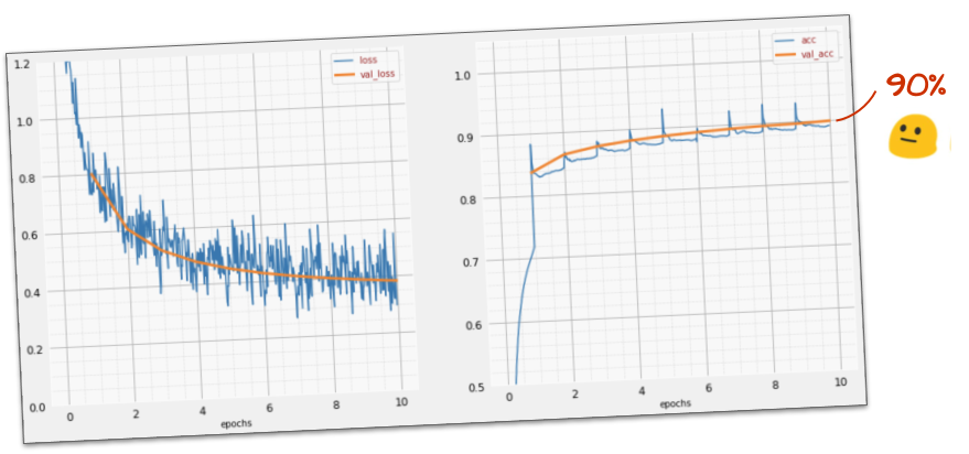
Monitoring Training Progress

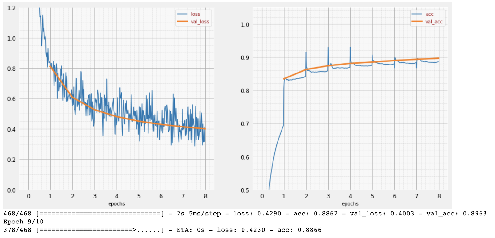
During training, we track two key metrics: accuracy and loss.

Accuracy (Right Plot):

• Percentage of correctly recognized digits.
• Should increase as training progresses.

Loss (Left Plot):

• Measures how “badly” the model performs.
• The goal is to minimize this value.
• Should decrease on both training and validation data.

X-axis: Epochs (iterations over entire dataset)

As our neural network trains, we want to monitor its progress. Neural network training is an iterative process where the model continually adjusts its internal weights and biases to improve its performance. The two primary metrics we observe during this process are accuracy and loss.

Accuracy is straightforward: it’s the proportion of correctly classified examples. Ideally, this should increase over time, indicating the model is getting better at its task.

Loss, on the other hand, is a numerical value that quantifies how “wrong” the model’s predictions are. Our training objective is to minimize this loss function. A decreasing loss on both the training and validation datasets is a strong indicator that the model is learning effectively and generalizing well. If the training loss continues to decrease but the validation loss starts to increase, that’s a sign of overfitting, which we’ll discuss later.

The X-axis in these plots represents epochs, where one epoch signifies one complete pass through the entire training dataset.

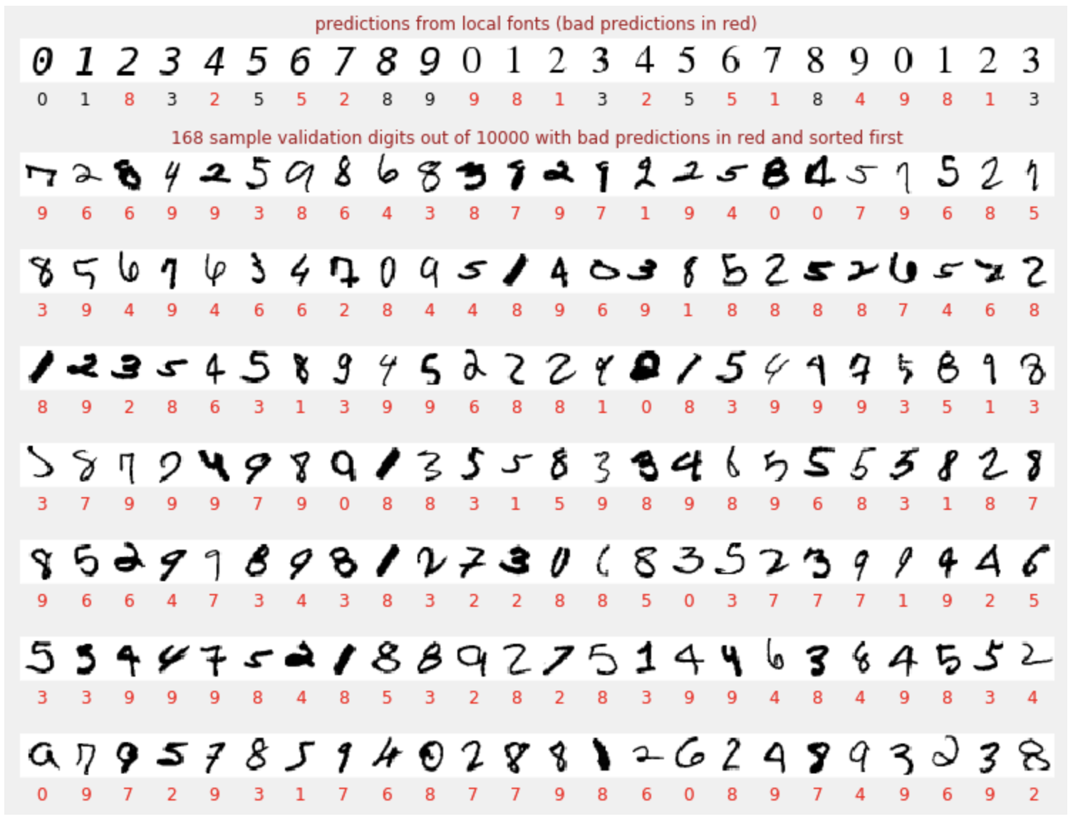
Making Predictions

After training, the model can predict digits it hasn’t seen.

This initial model reaches ~90% validation accuracy, meaning it still misclassifies 1000 out of 10,000 validation digits.

Caution

Even 90% accuracy leaves room for improvement, especially in critical ECE applications like medical imaging or autonomous systems.

Once training is complete, the true test of our model is its ability to make accurate predictions on new, unseen data. The visualization shows how our initial model performs on sample digits. Correct predictions are shown in black, and incorrect ones in red.

At 90% validation accuracy, the model is certainly respectable for a basic setup. However, in Many ECE applications, 90% might not be enough. For instance, if this were an autonomous driving system recognizing stop signs, a 10% error rate would be catastrophic. Even for digit recognition, if you’re processing millions of checks, a 10% error rate means a lot of manual corrections. This highlights why we constantly strive for higher accuracy and robustness in deep learning models.

Understanding Tensors: The Language of Data

In deep learning, data is represented as tensors. Tensors are multi-dimensional arrays, analogous to vectors and matrices.

• Grayscale Image (28x28 pixels): A 2D tensor (matrix) with shape [28, 28].

• Color Image (28x28 pixels, RGB): A 3D tensor with shape [28, 28, 3]. (Height, Width, Color Channels)

• Batch of Color Images (e.g., 128 images): A 4D tensor with shape [128, 28, 28, 3]. (Batch Size, Height, Width, Color Channels)

Note

The list of dimensions is called the “shape” of the tensor.

Understanding tensor shapes is crucial for building and debugging neural networks.

Before we dive into building models, it’s critical to understand how data is represented in deep learning. The fundamental data structure is the tensor. Think of a tensor as a generalization of a scalar (a single number), a vector (a 1D array), and a matrix (a 2D array) to an arbitrary number of dimensions.

For example, a simple grayscale handwritten digit image, which is 28x28 pixels, can be represented as a 2D tensor, or a matrix, with a shape of [28, 28]. If we had a color image, with red, green, and blue channels, it would need a third dimension for the color channels, giving it a shape like [28, 28, 3]. And often, we process images in batches to make training more efficient. So, a batch of 128 color images would become a 4D tensor with a shape of [128, 28, 28, 3].

The shape of a tensor tells you its dimensions, and understanding these shapes is absolutely crucial when designing neural network architectures and debugging issues. Incorrect tensor shapes are a very common source of errors.

Interactive Example: Image Compression Analogy

Let’s visualize how much information we retain when we reduce the “dimensions” of an image. This is analogous to how neural networks extract features.

viewof originalWidth = Inputs.range([100, 500], {value: 300, step: 10, label: "Original Width"});
viewof compressedWidth = Inputs.range([10, 100], {value: 50, step: 5, label: "Compressed Width"});

This interactive example uses an image compression analogy to illustrate how much information is retained as we reduce an image’s dimensions. In neural networks, particularly convolutional neural networks, we often downsample images (e.g., through pooling layers) to extract higher-level features and reduce computational load. By adjusting the “Compressed Width” slider, you can observe how a simplified representation of the image still captures its essence, much like how a neural network learns to represent complex patterns in a condensed form. This helps us understand the trade-offs between detail and efficiency in feature extraction.

Introduction to Neural Networks

Neural Networks are powerful computational models inspired by the human brain. They are used to learn complex patterns from data.

For ECE, neural networks are crucial in:

• Signal Processing: Noise reduction, feature extraction.
• Image Recognition: Object detection, medical imaging analysis.
• Control Systems: Adaptive control, robotics.

Welcome to this lecture on Neural Networks! In ECE, understanding how these networks work is becoming increasingly vital. We’ll explore their fundamental concepts and see how they apply directly to engineering problems you’ll encounter. Think of them as sophisticated tools for processing and understanding complex data, much like how you design circuits to process signals.

The Keras Sequential API

When building neural networks with TensorFlow and Keras, the Sequential API is a straightforward way to stack layers. This is ideal for models where layers have exactly one input tensor and one output tensor.

Example: Image Classifier using Dense Layers

model = tf.keras.Sequential([
    tf.keras.layers.Flatten(input_shape=[28, 28, 1]), # Flattens input images
    tf.keras.layers.Dense(200, activation="relu"),    # Hidden layer with ReLU
    tf.keras.layers.Dense(60, activation="relu"),     # Another hidden layer
    tf.keras.layers.Dense(10, activation='softmax')   # Output layer for 10 classes
])

model.compile(
    optimizer='adam',
    loss='categorical_crossentropy',
    metrics=['accuracy']
)
# Train the model
# model.fit(dataset, ...)

The Keras Sequential API is your go-to for building simple, layer-by-layer models. It’s like stacking different circuit components one after another. In ECE, you might think of each layer as a stage in a signal processing pipeline. The Flatten layer converts your 2D image data into a 1D vector, which is necessary for the Dense layers. Dense layers are fully connected, meaning every neuron in one layer connects to every neuron in the next. We’ll discuss activation functions like “relu” and “softmax” shortly.

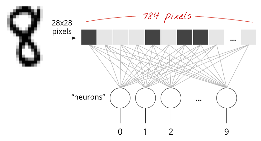
What is a Neuron? The Basic Building Block

The fundamental unit of a neural network is the neuron, a concept analogous to a processing unit in digital circuits.

Each neuron performs three main operations:

1. Weighted Sum: Multiplies each input by a corresponding weight and sums them up.
2. Bias Addition: Adds a bias constant to the weighted sum.
3. Activation: Passes the result through a non-linear activation function.

The weights (W) and biases (b) are the parameters learned during training. Initially, they are random and get adjusted to minimize error.

neuron.png

Tip

Think of weights as variable resistors and biases as constant voltage offsets in an analog circuit. The activation function is like a threshold detector or a non-linear amplifier.

The neuron is the basic computational element. It’s not unlike an operational amplifier with multiple inputs, where each input has a gain (weight) and an offset (bias), and the output is then shaped by a non-linear transfer function. These weights and biases are the “knobs” we turn during training to make the network learn.

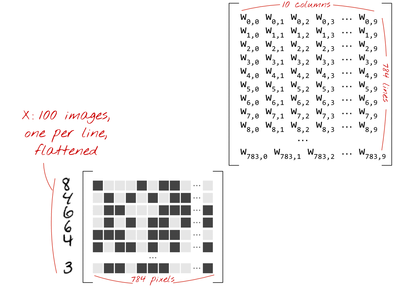
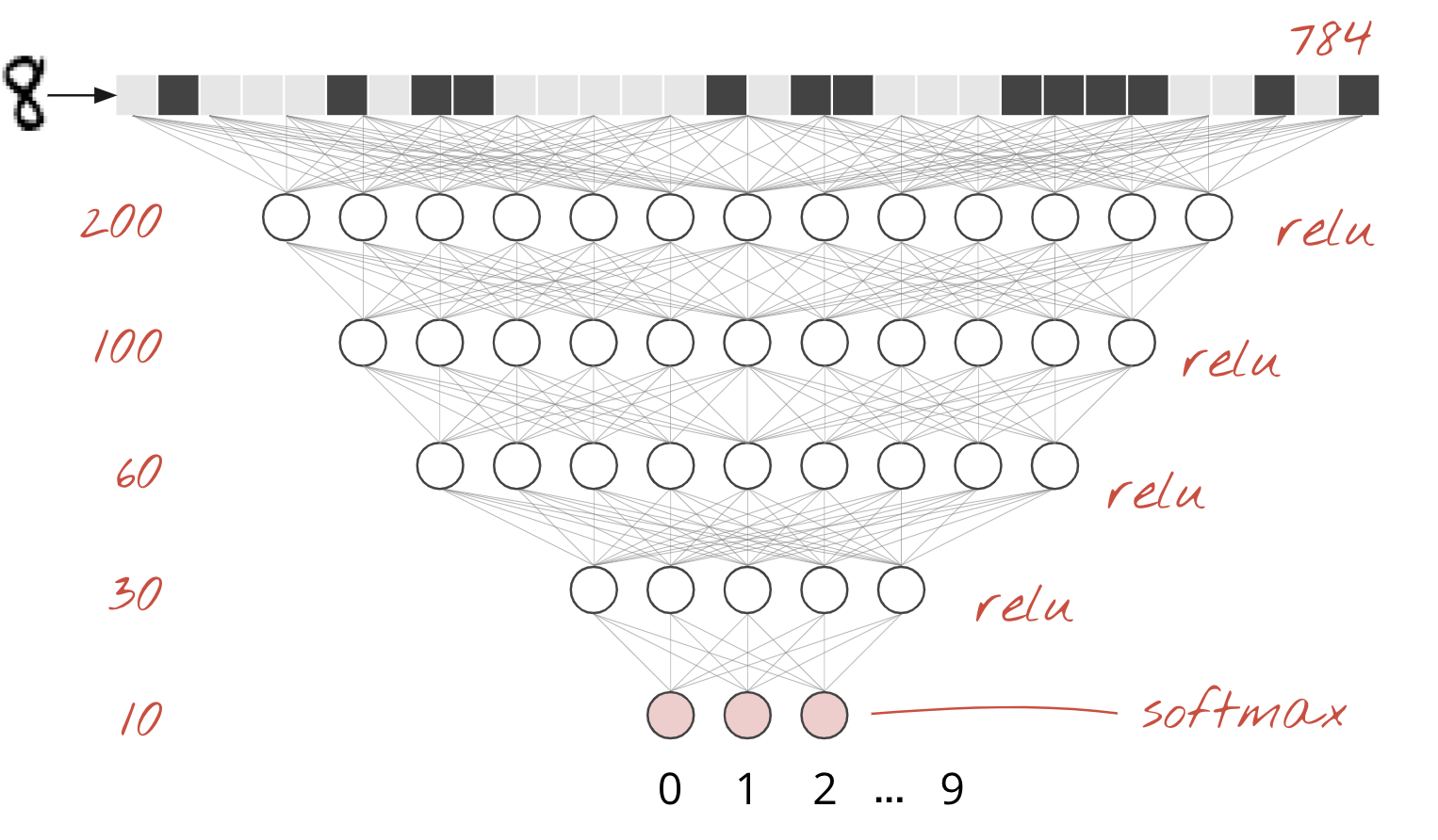
Single Dense Layer: MNIST Example

Let’s consider classifying handwritten digits from the MNIST dataset. Each image is 28x28 pixels grayscale.

The simplest neural network for this task uses 784 pixels (28x28) as inputs to a single dense layer.

This layer has 10 output neurons, one for each digit class (0-9).

Each of these 10 output neurons takes all 784 pixel values as input, performs a weighted sum, adds a bias, and applies an activation.

For MNIST, each 28x28 pixel image contains 784 individual pixel values. These 784 values become the direct inputs to the first layer of our neural network. Since we want to classify digits from 0 to 9, we need 10 output neurons, each corresponding to a specific digit. This diagram illustrates the “dense” or fully connected nature of this layer, where every input pixel influences every output neuron.

Matrix Multiplication for a Single Layer

A dense layer’s operations can be efficiently represented using matrix multiplication.

If X is a matrix of 100 images (each flattened to 784 pixels), and W is the weight matrix (784 inputs x 10 outputs), then:

\[ \text{Weighted Sums} = X \cdot W \]

\[ \text{Output} = \text{Activation}(X \cdot W + b) \]

Where b is the bias vector (10 elements), broadcasted across the 100 images.

Matrix Multiplication for a Single Layer

matmul.gif

In Keras, this is simplified:tf.keras.layers.Dense(10, activation='softmax')

The magic of linear algebra allows us to express thousands, or even millions, of neuron calculations as simple matrix multiplications. This is incredibly efficient for modern hardware like GPUs, which are optimized for these operations. X would be a 100x784 matrix, and W would be a 784x10 matrix. The product X \cdot W would then be a 100x10 matrix, where each row represents the 10 neuron outputs for one of the 100 images.

Going Deep: Chaining Layers

“Deep learning” refers to using multiple hidden layers. Each layer computes weighted sums of the outputs of the previous layer.

This architecture allows the network to learn progressively more complex and abstract features from the raw input data.

For example, early layers might detect edges or simple shapes, while later layers combine these to recognize parts of objects or entire objects.

The choice of activation function is critical and typically changes only for the very last layer in a classifier.

Going Deep: Chaining Layers

fba0638cc213a29.png

“Going deep” is like adding more stages to a complex signal processing pipeline, where each stage refines the information from the previous one. In image processing, the first layer might learn to identify basic lines or corners, while the second layer might combine these to detect ears or eyes, and final layers assemble these into a full face recognition. This hierarchical learning is a key advantage of deep networks.

Activation Functions: ReLU and Softmax

Activation functions introduce non-linearity, allowing neural networks to learn complex, non-linear relationships in data.

Sigmoid

• The most classical
• Used on intermediate layers

Rectified Linear Unit (ReLU)

\(f(x) = \max(0, x)\)

• Most popular activation for hidden layers.
• Simple and computationally efficient.
• Helps prevent vanishing gradients.

Softmax

\[ \sigma(z_i) = \frac{e^{z_i}}{\sum_{j=1}^K e^{z_j}} \]

• Used in the output layer of multi-class classifiers.
• Converts logits into probabilities that sum to 1.

sigmoid.png

relu.png

Non-linearity is crucial. Without it, stacking layers would just result in another linear transformation, essentially a single layer. ReLU is like a simple switch: if the input is positive, it passes it; otherwise, it stops it. Softmax is a smart way to get probabilities out of our network for classification. For instance, if you have ten possible digit classes, Softmax ensures that the network’s output is a set of ten probabilities that add up to one, indicating the likelihood of the input belonging to each class.

Softmax in Action: Interactive Example

Adjust the Logit Value for a single class and observe how Softmax normalizes probabilities. Here, we simulate 10 classes, with one Logit Value adjusted at a time.

viewof logit_val = Inputs.range([0, 10], {step: 0.1, value: 5, label: "Logit Value for Class 0 (others fixed at 1.0)"});

This interactive example demonstrates the power of Softmax. Notice how even a small increase in one logit value can significantly boost its corresponding probability, while simultaneously reducing the probabilities of other classes to ensure their sum remains 1. This is critical for making clear, probabilistic predictions in classification tasks.

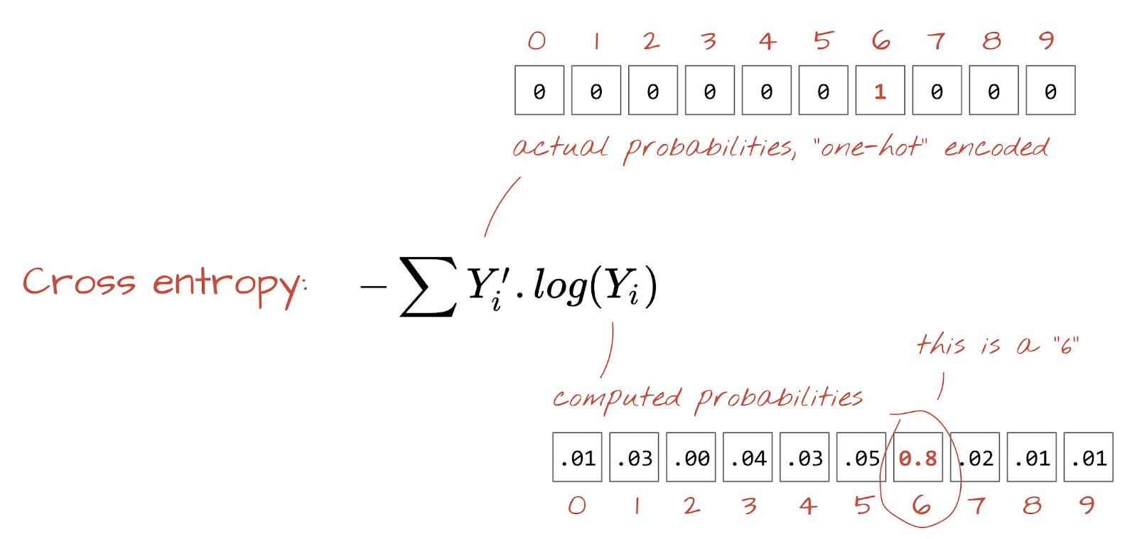
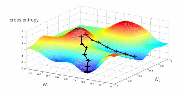
Loss Function: Cross-Entropy

To train a neural network, we need to measure how “wrong” its predictions are compared to the true labels. This measure is called the loss function.

For multi-class classification, Cross-Entropy Loss is the standard.

\[ H(p, q) = - \sum_{i=1}^{K} p_i \log(q_i) \]

Where: * \(p_i\) is the true probability for class \(i\) (1 for the correct class, 0 otherwise). * \(q_i\) is the predicted probability for class \(i\) (output of softmax). * \(K\) is the number of classes.

Note

Cross-entropy loss heavily penalizes incorrect high-confidence predictions, guiding the network to both be correct and confident.

Loss Function: Cross-Entropy

cross_entropy.png

The loss function is our feedback mechanism. It tells us how far off our network’s predictions are from the ground truth. Cross-entropy is particularly effective because it’s not just about getting the right answer; it’s also about how confident the network is when it’s right or wrong. Misclassifying an image with high confidence leads to a very large penalty, forcing the network to learn better.

Training: Gradient Descent

“Training” a neural network means iteratively adjusting its weights and biases to minimize the loss function. This is achieved using an optimization algorithm called Gradient Descent.

1. Compute Gradient: Calculate the partial derivatives of the loss function with respect to every weight and bias. This “gradient” vector points in the direction of the steepest increase of the loss.
2. Update Parameters: Adjust weights and biases in the opposite direction of the gradient, typically by a small step size called the learning rate.

\[ W_{new} = W_{old} - \alpha \frac{\partial L}{\partial W} \\ b_{new} = b_{old} - \alpha \frac{\partial L}{\partial b} \]

This process is repeated over many epochs (passes through the entire dataset).

Training: Gradient Descent

gradient_descent.png

Gradient descent is like a guided search. Imagine you’re blindfolded on a mountainous landscape (the loss function surface) and you want to find the lowest point. You feel the slope around you (compute the gradient) and take a small step downhill. You repeat this until you reach a valley. The ‘learning rate’ determines how big a step you take. Too large, and you might overshoot the minimum; too small, and it takes too long to converge.

Mini-Batching and Momentum

To improve training efficiency and stability:

Mini-Batching

• Instead of computing the gradient for one image at a time, we use a batch (e.g., 32, 64, or 128 images).
• Provides a more stable and representative gradient estimate.
• Leverages highly optimized matrix operations on GPUs/TPUs.

Momentum

• Adds a fraction of the previous update vector to the current update.
• Helps overcome local minima, saddle points, and speeds up convergence in relevant directions.

Mini-Batching and Momentum

saddle_point.png

Illustration: A saddle point, where the gradient is zero but not a true minimum in all directions.

Mini-batching is a practical optimization. Imagine getting directions from one person versus getting an averaged direction from a group of people; the latter is usually more reliable. Momentum, on the other hand, gives the optimization process inertia. It prevents the optimizer from getting stuck in “saddle points”—flat regions in the loss landscape that are not true minima. This is crucial for navigating high-dimensional spaces effectively.

Glossary of Key Terms

• Batch/Mini-batch: A subset of the training data used in one iteration of gradient descent.
• Cross-Entropy Loss: A common loss function for classification tasks, measuring dissimilarity between predicted and true probability distributions.
• Dense Layer: A layer where each neuron is connected to every neuron in the preceding layer.
• Features: The input attributes or data points fed into a neural network.
• Labels: The correct outputs or target values in supervised learning.
• Learning Rate: A hyperparameter controlling the step size during gradient descent.
• Logits: The raw, unnormalized outputs of a neural network layer before being passed through an activation function like softmax.
• Loss Function: A function that quantifies the error between predicted outputs and true labels.
• Neuron: The fundamental computational unit of a neural network.
• One-Hot Encoding: A categorical variable representation where each category is a binary vector (e.g., [0,0,1,0] for class 3 of 4).
• ReLU (Rectified Linear Unit): A popular activation function, \(f(x) = \max(0, x)\).
• Sigmoid: An S-shaped activation function, \(f(x) = 1 / (1 + e^{-x})\).
• Softmax: An activation function that converts a vector of numbers into a probability distribution.
• Tensor: A generalization of vectors and matrices to an arbitrary number of dimensions.

This glossary provides a quick reference for the key terms we’ve covered. Understanding these terms is foundational for further study and application of machine learning in ECE.

Diving into the Code (Part 1)

Now, let’s dissect the code from the keras_01_mnist.ipynb notebook. Understanding each section is key to building and modifying models.

Note

Follow along in the Colab notebook if you can!

We’ll cover core components: - Model Parameters and Imports - Data Preparation with tf.data.Dataset - Building a Keras Sequential Model - Training and Validation - Visualizing Predictions

Model Parameters and Imports

These initial cells set up the environment and define global constants.

Parameters Cell:

Sets values for:

• BATCH_SIZE: Number of samples processed per gradient update.
• EPOCHS: Number of complete passes through the training dataset.
• GCS_PATTERN: Location of MNIST data files on Google Cloud Storage.

Imports Cell:

Imports necessary libraries:

• tensorflow (tf): Core Deep Learning framework.
• numpy (np): For numerical operations (especially tensor manipulation).
• matplotlib.pyplot (plt): For plotting and visualization.

# Example of Parameters
BATCH_SIZE = 64
EPOCHS = 5
GCS_PATTERN = "gs://cloud-tpu-datasets/mnist/mnist_{}.tfrec"

print(f"Batch Size: {BATCH_SIZE}")
print(f"Epochs: {EPOCHS}")

# Example of Imports
import tensorflow as tf
import numpy as np
import matplotlib.pyplot as plt

print("TensorFlow version:", tf.__version__)
print("NumPy version:", np.__version__)

The first crucial step in any machine learning project is to set up our environment and define key hyper-parameters.

The “Parameters” cell defines values like BATCH_SIZE, which controls how many training examples are processed together before the model’s weights are updated. EPOCHS determines how many full iterations the model makes over the entire training dataset. The GCS_PATTERN indicates where our MNIST dataset is stored, in this case, on Google Cloud Storage.

The “Imports” cell brings in all the necessary Python libraries. tensorflow is our backbone for deep learning. numpy is essential for numerical operations and efficient array manipulation, which is fundamental to working with tensors. Lastly, matplotlib.pyplot is indispensable for visualizing our data, training progress, and results.

Data Preparation with tf.data.Dataset

The tf.data.Dataset API is powerful for building efficient data pipelines. It handles loading, parsing, and preprocessing data, especially at scale.

Key Steps:

1. Load Fixed-Length Records: Images and labels are stored in tfrec files. We decode raw byte strings into images (float32, normalized 0-1) and flatten them.

   imagedataset = tf.data.FixedLengthRecordDataset(image_filename, 28*28, header_bytes=16)

2. read_image Function: Parses byte strings into float32, normalizes pixels (0-1), and reshapes to [28*28] (flattened for initial dense layer).

   def read_image(tf_bytestring):
       image = tf.io.decode_raw(tf_bytestring, tf.uint8)
       image = tf.cast(image, tf.float32)/256.0
       image = tf.reshape(image, [28*28])
       return image

Preparing data efficiently is as important as designing the neural network itself. TensorFlow’s tf.data.Dataset API is specifically designed for this, allowing us to build highly optimized input pipelines.

The MNIST dataset images and labels are stored in a specialized format known as tfrec (TFRecord) files. The FixedLengthRecordDataset is used to read these files, assuming each record (image) has a fixed length. We also skip a header of 16 bytes.

The read_image function is crucial. Raw image data comes as bytes (tf.uint8). We cast this to tf.float32 because neural networks generally prefer floating-point inputs. We then normalize the pixel values from the [0, 255] range to [0, 1] by dividing by 256. Finally, we reshape the 2D 28x28 image into a 1D vector of 28*28 = 784 pixels because our initial single-layer model expects a flattened input.

Data Preparation (Cont.): Pipeline Operations

After parsing, we apply various transformations to optimize the dataset for training:

1. Mapping & Zipping:

• Apply read_image to all images using .map().
• Do similar steps for labels.
• Combine images and labels using .zip(): dataset = tf.data.Dataset.zip((imagedataset, labelsdataset))

2. Optimizations:

• .cache(): Store dataset in RAM for faster epoch transitions (for small datasets).
• .shuffle(buffer_size): Randomize training order to prevent batch order biases.
• .repeat(): Loop the dataset indefinitely for multiple epochs.
• .batch(batch_size): Group samples into mini-batches for efficient processing.
• .prefetch(tf.data.experimental.AUTOTUNE): Overlap data preprocessing and model execution to keep the GPU busy.

Once individual images and labels are read and decoded, we build the full data pipeline using a sequence of tf.data.Dataset operations.

First, we use .map() to apply our read_image function across the entire image dataset. We perform analogous steps for the labels, then use .zip() to pair each image with its corresponding label, forming a dataset of (image, label) pairs.

Next come the crucial optimizations for training:

• .cache() stores the prepared dataset in RAM after the first epoch, eliminating redundant processing in subsequent epochs, which is excellent for smaller datasets like MNIST.
• .shuffle() randomizes the order of examples within a specified buffer. This prevents the model from learning spurious patterns related to the order of appearance in the dataset.
• .repeat() ensures that the dataset loops indefinitely, so we can train for multiple epochs without explicitly re-initializing the data pipeline.
• .batch() groups individual examples into mini-batches. This is fundamental for efficient training, as gradient updates are typically computed over batches, not individual examples.
• .prefetch(tf.data.experimental.AUTOTUNE) is a performance booster. It allows the data pipeline to prepare the next batch of data on the CPU while the current batch is being processed by the GPU, maximizing hardware utilization.

Building a Keras Sequential Model: The 1-Layer Network

Our first model is a simple, single-layer dense neural network.

Model Definition:

• We use tf.keras.Sequential for a linear stack of layers.
• tf.keras.layers.Input(shape=(28*28,)): Defines the input shape (784-element flattened vector).
• tf.keras.layers.Dense(10, activation='softmax'):
  • 10 neurons: One for each digit class (0-9).
  • 'softmax' activation: Outputs a probability distribution over the 10 classes, summing to 1. (The highest probability indicates the predicted class.)

Now, let’s get to the heart of the neural network: the model itself. Keras provides a very intuitive API for building models. For simple, layer-by-layer architectures, tf.keras.Sequential is perfect.

Our first model is remarkably simple:

1. Input Layer: We explicitly define the input shape using tf.keras.layers.Input. Since we flattened our 28x28 images, the input to this layer is a 1D vector of 784 pixels.
2. Dense Layer: This is the core of our model. A “Dense” layer (also known as a fully connected layer) means every neuron in this layer is connected to every neuron in the previous layer.
   • It has 10 neurons, one for each output class (digits 0 through 9).
   • The activation='softmax' is critical for classification tasks. Softmax converts the raw output of the neurons into a probability distribution, ensuring that all 10 output values are positive and sum up to 1. The class with the highest probability is our model’s prediction.

Compiling the Model

Before training, the model needs to be compiled. Compilation configures key aspects of the training process.

model.compile(optimizer='sgd',
              loss='categorical_crossentropy',
              metrics=['accuracy'])

• optimizer='sgd' (Stochastic Gradient Descent): The algorithm used to update the model’s weights based on the loss. SGD is a foundational optimizer for neural networks.
• loss='categorical_crossentropy': The loss function measures the discrepancy between predicted and true class probabilities. Categorical crossentropy is standard for multi-class classification when labels are one-hot encoded.
• metrics=['accuracy']: Additional metrics to monitor during training and evaluation. 'accuracy' measures the percentage of correct predictions.

Compiling the model is like setting up the engine and navigation system before going on a trip. It’s where we define how the model will learn.

1. Optimizer: The optimizer is the algorithm that adjusts the weights of the neural network during training to minimize the loss function. ‘SGD’, or Stochastic Gradient Descent, is the simplest and a very common optimizer. It makes small, iterative adjustments to the weights based on the gradient of the loss function with respect to the weights.

2. Loss Function: The loss function quantifies how ‘bad’ our model’s predictions are compared to the true labels. For multi-class classification problems like MNIST where each input belongs to exactly one class out of many, categorical_crossentropy is the standard choice. It penalizes incorrect predictions more heavily when the model was very confident in its wrong answer.

3. Metrics: Metrics are used to monitor the training and validation process. While the loss function guides the optimization, metrics provide a more human-interpretable measure of performance. ‘Accuracy’ is intuitive: it’s the proportion of correctly classified examples.

Model Summary & Training Utility

After compilation, we can inspect the model’s architecture.

model.summary():

Prints a detailed overview of the model:

• Layers (type, output shape).
• Number of trainable parameters in each layer.
• Total parameters in the model.

This is invaluable for debugging and understanding model complexity.

PlotTraining Callback:

A custom utility (from the notebook) to visualize training curves dynamically. It shows loss and accuracy for both training and validation sets in real-time.

import tensorflow as tf
# Define a simple model for demonstration
model_summary_demo = tf.keras.Sequential([
    tf.keras.layers.Input(shape=(28*28,)), # For MNIST, inputs are 784-element vectors
    tf.keras.layers.Dense(10, activation='softmax') # 10 output classes
])

# Simulate compile for summary to show expected parameters
model_summary_demo.compile(optimizer='sgd', loss='categorical_crossentropy', metrics=['accuracy'])

# Print the model summary
model_summary_demo.summary()

Before we start training, it’s good practice to inspect the model’s structure.

model.summary() is an extremely useful Keras utility. It outputs a table showing each layer, its output shape, and the number of parameters it has.

• Output Shape: This tells us the shape of the tensor outputted by each layer. For our Dense layer with 10 neurons, the output shape is (None, 10), where None indicates the batch size, which can vary.
• Trainable parameters: For the Dense layer, this is (input_features + 1) * output_neurons. In our case (784 + 1) * 10 = 7850. The +1 accounts for the bias term for each neuron.

The PlotTraining callback, though custom, is typical of utilities used to provide visual feedback during training. It helps identify issues like overfitting early on.

Training and Validation

The model.fit() function is where the actual learning takes place.

model.fit(training_dataset,
          steps_per_epoch=steps_per_epoch,
          epochs=EPOCHS,
          validation_data=validation_dataset,
          validation_steps=1,
          callbacks=[plot_training])

• training_dataset: The preprocessed dataset used for learning.
• steps_per_epoch: Number of batches per epoch (total training samples / batch size).
• epochs: Total number of times the model iterates over the entire training data.
• validation_data: The unseen dataset used to evaluate performance after each epoch.
• validation_steps: Number of batches from validation_data to run per validation round.
• callbacks: List of custom functions executed at various stages of training (e.g., plot_training).

With the model defined and compiled, we’re ready for the most exciting part: training! This is done using the model.fit() method.

• training_dataset: This is our tf.data.Dataset pipeline for the training data.
• steps_per_epoch: Since we used dataset.repeat(), the data pipeline could theoretically run forever. steps_per_epoch tells Keras how many batches constitute one “epoch” or one full pass through our conceptual dataset. It is typically calculated as total_training_samples / BATCH_SIZE.
• epochs: As defined in our parameters, this is the total number of epochs the model will train for.
• validation_data: Here, we pass our tf.data.Dataset pipeline for the validation data. Keras automatically evaluates the model on this data at the end of each epoch.
• validation_steps: Similar to steps_per_epoch, this specifies how many validation batches to process during each validation run.
• callbacks: This is a list where we can include custom functions that execute during training. Our plot_training callback is a great example, providing real-time visualization of metrics.

Visualizing Predictions

After training, we use model.predict() to evaluate the model on new inputs.

probabilities = model.predict(font_digits, steps=1)
predicted_labels = np.argmax(probabilities, axis=1)

• model.predict(input_data): Generates output predictions for the input samples. For a classification model with softmax activation, it returns a 2D array where each row is a probability distribution over the classes for one input. (e.g., [[0.01, 0.05, ..., 0.90, ..., 0.02], ...])
• np.argmax(probabilities, axis=1): Converts the probability distributions into a single predicted class label.
  • np.argmax(): Returns the index of the maximum value.
  • axis=1: Specifies to find the maximum along the “class” dimension (i.e., for each image, find the class with the highest probability).

Visualizing Predictions

Note

This simple 1-layer model already achieves ~90% accuracy! But we can do much better.

Adding Layers: Going Deeper

To improve our model’s accuracy beyond 90%, we need to add more layers. This allows the network to learn more complex, hierarchical features.

The Concept of Depth

• A deeper network can model non-linear relationships more effectively.
• Each hidden layer learns increasingly abstract representations of the input data.

Our single-layer neural network achieved about 90% accuracy, which is a good baseline, but not yet sufficient for many real-world ECE applications. To push this accuracy higher, the most intuitive next step is to make our neural network deeper by adding more layers.

Why go deeper? Deep networks are powerful because they can learn hierarchies of features. For image recognition, the first layer might learn simple edges or lines. A second layer might combine these to recognize shapes like circles or corners. A third layer might combine shapes to recognize parts of digits, and so on. This hierarchical learning allows deep networks to model very complex, non-linear relationships in the data, far beyond what a single layer can achieve.

Activation Functions Revisited

While softmax is for the output layer of a classifier, hidden layers need different activation functions.

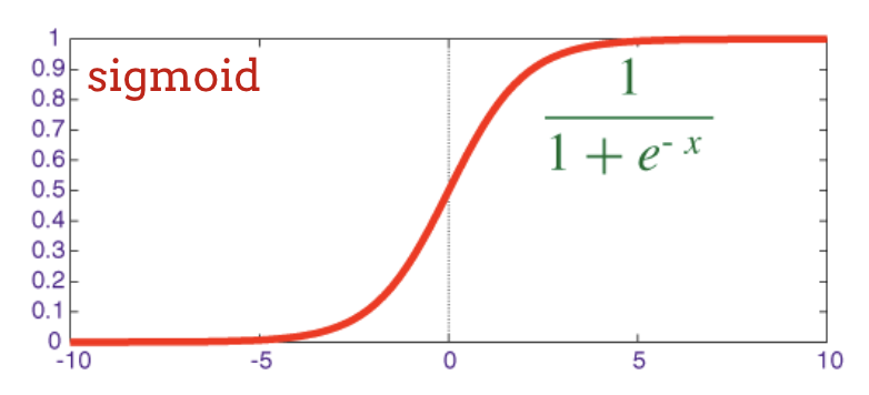
Sigmoid Activation Function

For intermediate (hidden) layers, the sigmoid function is a classical choice:

\[ \sigma(x) = \frac{1}{1 + e^{-x}} \]

• Output Range: Maps any input to a value between 0 and 1.
• Interpretation: Can be seen as a “soft” switch, where values close to 0 or 1 indicate strong decisions.
• Historical Significance: Widely used in early neural networks.

Plot of the Sigmoid Function

When we add more layers, we introduce hidden layers between the input and output. Each neuron in these hidden layers needs an activation function to introduce non-linearity into the network. Without non-linearity, no matter how many layers you add, the neural network would only be able to learn linear relationships, limiting its power.

While softmax is perfect for the final classification layer, where we need probabilities for multiple classes, sigmoid is a classic choice for hidden layers. The sigmoid function squashes any input value into a range between 0 and 1. This can be interpreted as the “activation” strength of a neuron. Historically, sigmoid was one of the most popular activation functions, but we will soon see more effective alternatives for deeper networks.

Designing a Deeper Model

Let’s expand our simple model by adding two hidden Dense layers with sigmoid activation.

model = tf.keras.Sequential(
    [
        tf.keras.layers.Input(shape=(28*28,)),        # Input Layer
        tf.keras.layers.Dense(200, activation='sigmoid'), # Hidden Layer 1
        tf.keras.layers.Dense(60, activation='sigmoid'),  # Hidden Layer 2
        tf.keras.layers.Dense(10, activation='softmax')   # Output Layer
    ]
)
# (Compilation and training code follows)

• Hidden Layer 1: 200 neurons with sigmoid activation.
• Hidden Layer 2: 60 neurons with sigmoid activation.
• Output Layer: Remains 10 neurons with softmax for classification.

Note

Notice the increase in the number of parameters with multiple layers. Run this model in the Colab notebook.

Here’s how we’d implement a deeper network in Keras. We simply add more tf.keras.layers.Dense components to our Sequential model.

• We start with our Input layer, still expecting the flattened 784-pixel vector.
• Then we add tf.keras.layers.Dense(200, activation='sigmoid'). This layer has 200 neurons, processing the 784 inputs and producing 200 outputs. The sigmoid activation squashes these outputs between 0 and 1.
• Next, another hidden layer: tf.keras.layers.Dense(60, activation='sigmoid'). This layer takes the 200 outputs from the previous layer as its input, processes them with 60 neurons, and outputs 60 values.
• Finally, our output layer remains the same: tf.keras.layers.Dense(10, activation='softmax'), producing the 10 probabilities for digit classification.

By running model.summary() again, you’ll see a significant increase in the total number of trainable parameters. This increased capacity should, in theory, allow the a model to learn more intricate patterns.

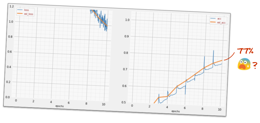
Unexpected Behavior: What Happened?

Despite adding layers and parameters, the model doesn’t always improve as expected.

• High Loss: The training loss and validation loss are extremely high.
• Low Accuracy: Accuracy barely increases above random guessing (around 10%).

Warning

More parameters don’t automatically mean better performance. Deeper networks introduce new challenges!

After running the deeper model in the Colab notebook, you might observe a surprising and discouraging result: the model performs worse than our single-layer network. The training and validation loss remain prohibitively high, and the accuracy barely moves beyond 10%, which is what you’d expect from random guessing among 10 classes.

This outcome clearly illustrates an important point in deep learning: simply adding more layers and parameters isn’t a silver bullet. Deeper networks come with their own set of challenges. This particular issue with sigmoid activations in deep networks is a classic problem known as the vanishing gradient problem, which we will discuss next. The sigmoid function, especially for inputs far from zero, has very small gradients. In a deep network, these small gradients are multiplied together as they propagate backward through the layers, causing them to “vanish” by the time they reach earlier layers. This prevents the weights in those earlier layers from being updated effectively, stalling learning.

Why Did the Deeper Model Fail? The Vanishing Gradient Problem

The sigmoid activation function can hinder learning in deep networks.

The Problem:

• The gradient (derivative) of the sigmoid function is very small for inputs far from 0.
• In a deep network, these small gradients are multiplied together during backpropagation.
• This causes gradients to “vanish” as they propagate back to earlier layers.

Consequence for ECE:

• Early layers’ weights are hardly updated.
• The network struggles to learn useful features from the input.
• Training stalls, leading to poor performance.

Important

This is a common issue with traditional activation functions like sigmoid and tanh in deep architectures.

Special Care for Deep Networks

The “AI winter” of the 80s and 90s was partly due to the challenges of training deep networks. Modern deep learning thrives due to “dirty tricks” that ensure convergence.

Overcoming Deep Network Challenges

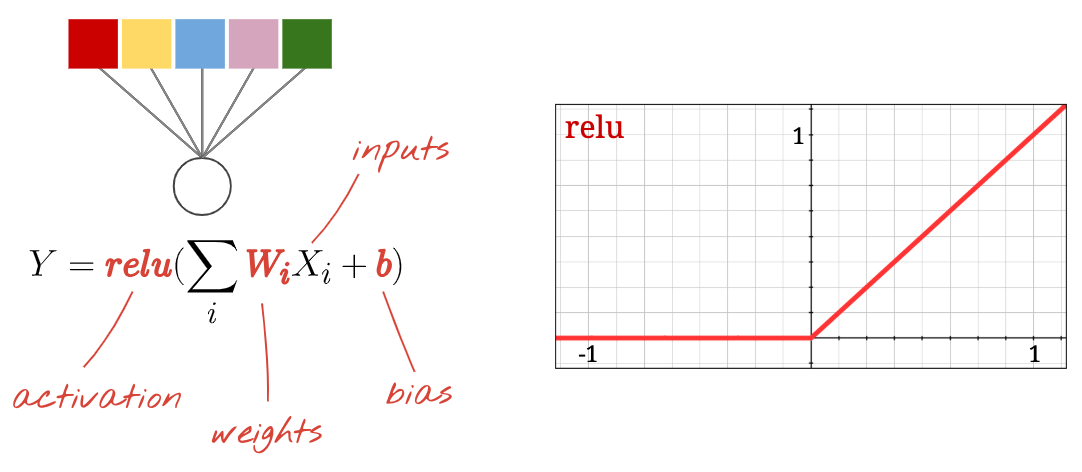
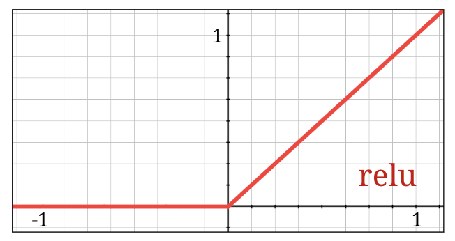
• RELU Activation: A simple yet powerful non-linearity.
• Better Optimizers: Algorithms that navigate complex loss landscapes.
• Careful Initialization: Setting initial weights to facilitate learning.
• Numerical Stability: Ensuring calculations don’t crash.

As we saw, simply adding more layers to a network with sigmoid activations often leads to poor performance, a problem that significantly contributed to the “AI winter.” However, thanks to a few crucial mathematical and algorithmic advancements, deep neural networks, even with 20, 50, or hundreds of layers, can now be trained effectively. These “dirty tricks,” as the source calls them, address the fundamental challenges of deep network convergence and have been instrumental in the recent resurgence of deep learning. We’ll explore these techniques now.

RELU Activation: The Modern Choice

The sigmoid function’s vanishing gradients made it problematic for deep networks. The Rectified Linear Unit (RELU) is the de-facto standard activation today.

\[ \text{ReLU}(x) = \max(0, x) \]

• Simplicity: Returns x for positive inputs, 0 for negative inputs.
• Gradient: Has a constant gradient of 1 for positive inputs.
• Benefits for ECE:
  • Mitigates vanishing gradient problem.
  • Speeds up convergence.
  • Computationally much cheaper than sigmoid/tanh.

Plot of the ReLU Function

Note

Replace activation='sigmoid' with activation='relu' in hidden layers. The output layer retains softmax for classification.

The sigmoid activation function was historically significant, but its propensity to squash values between 0 and 1 resulted in very small gradients, leading to the vanishing gradient problem in deep networks. The solution that revolutionized deep learning is surprisingly simple: the Rectified Linear Unit, or ReLU.

ReLU(x) simply outputs x if x is positive, and 0 if x is negative.

• Simplicity: This piece-wise linear function is incredibly simple to compute.
• Gradient: Crucially, its gradient is 1 for positive inputs and 0 for negative inputs. This 1 gradient for a large portion of its domain means that gradients can flow much more effectively through the network without vanishing, thereby addressing the core problem. This allows deeper networks to learn much faster and more effectively.
• Computational Efficiency: ReLU is also much faster to compute than exponentials (in sigmoid) or hyperbolic tangents, which speeds up training significantly.

For our ECE applications where efficiency and convergence are critical, ReLU is the go-to choice for hidden layers. Remember to keep softmax for the final output layer in classification tasks.

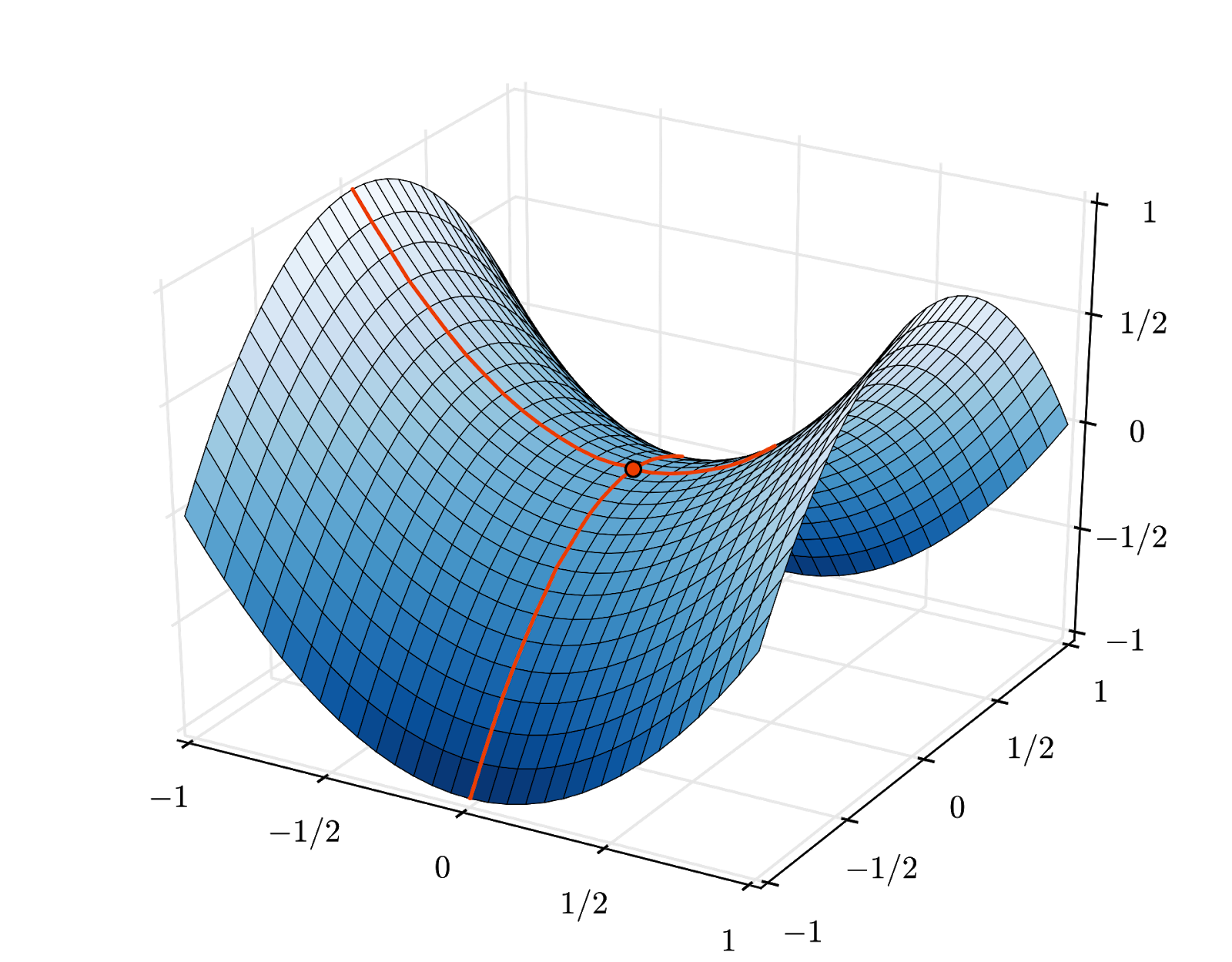
Better Optimizers: Beyond SGD

Stochastic Gradient Descent (SGD) can get stuck in “saddle points” in high-dimensional spaces.

Modern optimizers are more robust and efficient.

Saddle Points:

• Points in the loss landscape where the gradient is zero, but it’s not a true minimum.
• SGD can get stuck here, preventing further learning.

Adaptive Optimizers:

• Use concepts like “momentum” and “adaptive learning rates” for each parameter.
• Help the model “sail past” saddle points and converge faster.
• Examples: Adam, RMSprop, Adagrad.

Keras Implementation:

Update the optimizer in model.compile:

model.compile(optimizer='adam', # Use Adam optimizer
              loss='categorical_crossentropy',
              metrics=['accuracy'])

Tip

Adam is widely considered a good default choice for most deep learning tasks.

While SGD is foundational, its simplicity can be a drawback in complex, high-dimensional loss landscapes, which are typical for deep neural networks. One significant issue is saddle points. Imagine a mountain pass where the terrain flattens out. The gradient at this point is zero, just like at a local minimum. SGD, looking only at the immediate gradient, would mistakenly think it’s reached a minimum and stop, even if there are lower points to explore.

Modern optimizers like Adam, RMSprop, and Adagrad address this by incorporating more sophisticated mechanics. They often include:

• Momentum: This helps the optimizer build up speed in a consistent direction and overshoot small local minima or saddle points, like a ball rolling down a hill that doesn’t just stop at the first dip.
• Adaptive Learning Rates: Instead of using a single learning rate for all parameters, these optimizers maintain a separate learning rate for each network weight, adapting it based on the historical gradients. This allows for faster learning in some dimensions and more cautious steps in others.

By simply changing our optimizer from 'sgd' to 'adam' in Keras, we leverage these advanced techniques immediately, leading to faster and more reliable convergence.

Weight Initialization & Numerical Stability

Two critical, often hidden, factors for stable deep network training.

1. Random Initializations:

• How the network’s weights and biases are set before training begins.
• Poor initialization can lead to slow convergence or vanishing/exploding gradients.
• Keras Default: Uses 'glorot_uniform' (also known as Xavier uniform).
  • Designed to keep activation values and gradients roughly in the same scale across layers.
  • No action needed: Keras handles this optimally by default.

2. Numerical Stability (NaNs):

• Categorical crossentropy involves log(). If input to log is 0, it’s NaN (Not a Number).
• softmax output (probabilities) can be numerically 0 in float32 despite being mathematically non-zero.
• Keras Solution: tf.keras.losses.CategoricalCrossentropy(from_logits=True)
  • Computes softmax and crossentropy together in a numerically stable way.
  • No action needed: Keras handles this automatically when softmax is the last activation and categorical_crossentropy is the loss.

Beyond activations and optimizers, two more subtle but profoundly important aspects of deep learning convergence are weight initialization and numerical stability.

1. Weight Initialization: The starting values of a neural network’s weights and biases are surprisingly critical. If they are too large, activations might saturate; if too small, gradients might vanish. The goal is to initialize weights such that the activations and gradients flowing through the network remain in a reasonable range. Keras, by default, uses clever initialization schemes like 'glorot_uniform' (also known as Xavier uniform initialization), which attempts to balance the variance of activations and gradients across layers. The good news for us is that Keras usually “does the right thing” here, so we often don’t need to specify it manually.

2. Numerical Stability (NaNs): Our categorical_crossentropy loss function involves a logarithm. Mathematically, the softmax activation function produces probabilities that are strictly greater than zero (since it uses exponentials). However, in the finite precision world of float32 computer arithmetic, a very small positive number can be represented as 0. If log(0) occurs, the result is NaN (Not a Number), which crashes the training process. Keras smartly handles this by offering a version of categorical_crossentropy that optimally combines the softmax calculation with the cross-entropy loss in a numerically stable way, often internally using a from_logits=True argument when you specify 'softmax' and 'categorical_crossentropy'. This prevents those dreaded NaNs. Again, Keras typically manages this under the hood, so usually, no explicit action is required from us.

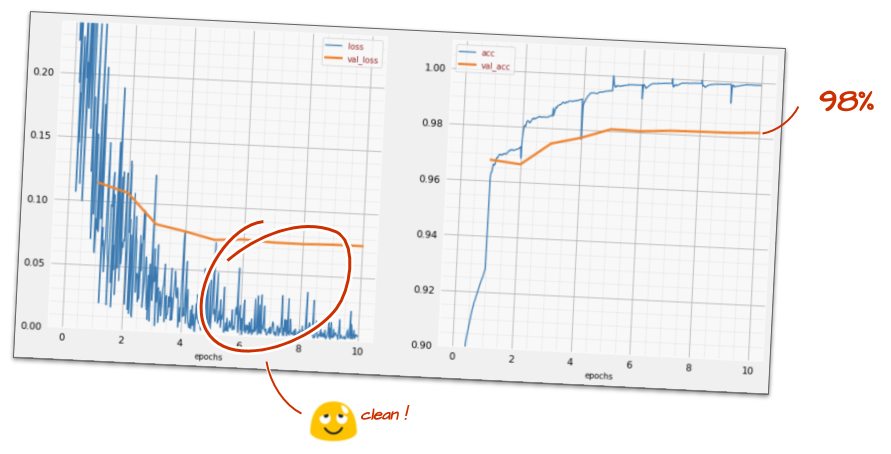
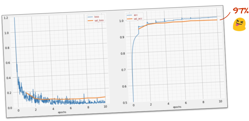
Success So Far: ~97% Accuracy!

With ReLU activation and the Adam optimizer, our deeper model should now converge effectively.

You should observe:

• Training and validation loss decreasing steadily.
• Training and validation accuracy climbing to around 97%.

This marks a significant improvement over the initial 90% and the failed deep sigmoid model.

We’re approaching our goal of “significantly above 99% accuracy!”

(Example of ~97% accuracy training curves)

Tip

If you’re stuck, refer to keras_02_mnist_dense.ipynb in the Colab repo.

After implementing ReLU activations in the hidden layers and switching to the Adam optimizer, you should see a dramatic improvement in your model’s performance. The training and validation curves for both loss and accuracy will now look much healthier, steadily converging. We’re now hitting around 97% accuracy, which is a major leap from our initial 90% and the failed sigmoid model. This demonstrates the critical importance of these “dirty tricks” in making deep networks viable. We’re definitely on the right track towards our ultimate goal!

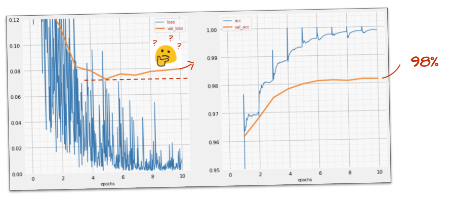
Learning Rate Decay: Fine-Tuning Convergence

Training too fast can lead to noisy convergence or even divergence. A learning rate decay schedule starts fast and slows down over time.

The Problem with High Learning Rates:

• Training curves become noisy.
• Validation metrics jump erratically (d4fd66346d7c480e.png).
• Model might jump over optimal solutions or oscillate.

The Solution:

• Start with a higher learning rate to explore the loss landscape quickly.
• Gradually decrease the learning rate as training progresses, allowing for finer adjustments and more stable convergence.
• Often exponential decay: \(LR = LR_0 \times \text{decay_rate}^{\text{epoch}}\)

Even with a powerful optimizer like Adam, simply using a fixed learning rate throughout training isn’t always optimal. Imagine searching for the lowest point in a valley. You might want to take large strides initially to cover ground quickly, but as you approach the bottom, you’d need smaller, more precise steps to find the exact lowest point without overshooting it.

In deep learning, the learning rate controls the step size of our optimizer. A very high learning rate can cause the model to bounce around the loss landscape without converging or even diverge. A very low learning rate can make training painfully slow.

The solution is learning rate decay. We start with a relatively high learning rate to make quick progress early on, and then gradually decrease it over epochs. This allows the model to fine-tune its weights as it gets closer to an optimal solution. Exponential decay is a common and effective schedule, where the learning rate shrinks by a constant factor after each epoch.

Implementing Learning Rate Decay with Keras

Keras makes it easy to add a learning rate scheduler using a callback.

1. Define the Decay Function: A Python function that calculates the learning rate for a given epoch.

import math
def lr_decay(epoch):
    return 0.01 * math.pow(0.6, epoch) # Exponential decay

This function starts at 0.01 and reduces it by 0.6 (60%) each epoch.

2. Create the Callback:

lr_decay_callback = tf.keras.callbacks.LearningRateScheduler(lr_decay, verbose=True)

verbose=True prints the learning rate at the start of each epoch.

3. Add to model.fit():

Include the lr_decay_callback in the list of callbacks.

model.fit(..., callbacks=[plot_training, lr_decay_callback])

Implementing Learning Rate Decay with Keras

Important

The lr_decay_callback must be added to the callbacks list for it to take effect.

Keras provides a flexible way to implement custom learning rate schedules using the tf.keras.callbacks.LearningRateScheduler.

1. Define the Decay Function: First, you define a Python function (like lr_decay here) that takes the current epoch number as input and returns the desired learning rate for that epoch. Our example uses an exponential decay, starting at 0.01 and multiplying by 0.6 (a 40% reduction) at each subsequent epoch.
2. Create the Callback: You then instantiate tf.keras.callbacks.LearningRateScheduler, passing your decay function to it. Setting verbose=True is helpful for debugging, as it prints the calculated learning rate at the beginning of each epoch.
3. Add to model.fit(): The final step is to include this lr_decay_callback in the callbacks list when you call model.fit(). Keras will then automatically call your function at the start of each epoch and update the optimizer’s learning rate accordingly.

The interactive plot generated by the plot_learning_rate utility demonstrates how the learning rate will decrease over the epochs according to our defined function. This visual confirms our strategy.

Impact of Learning Rate Decay: Cleaner Convergence

The effect of learning rate decay is often dramatic.

• Noise Reduction: Training curves become much smoother.
• Stable Validation: Validation accuracy and loss fluctuate less, showing cleaner convergence.
• Improved Accuracy: Sustained test accuracy can now be observed above 98%.

This technique is crucial for pushing models to higher performance ceilings.

(Training curves with learning rate decay)

The impact of implementing learning rate decay is usually quite significant and immediately visible in the training plots. You’ll notice that the training and validation curves, which might have been noisy and erratic before, become much smoother. This indicates that the model is making more stable and directed progress towards minimizing the loss.

More importantly, the validation accuracy, which is our true measure of generalization, becomes more stable and can push higher, often achieving levels above 98% in a consistent manner. This clearly shows that learning rate decay is not just a tweak but a fundamental technique for achieving robust and high-performing deep learning models. It helps the optimizer fine-tune the weights effectively as the model approaches optimal solutions.

7. Overfitting and Dropout

Even with a deeper network, ReLU, Adam, and learning rate decay, we often hit a wall around 98% accuracy. This is frequently due to overfitting.

The Signs of Overfitting

• Validation loss increases: While training loss continues to decrease.
• Validation accuracy plateaus or drops: While training accuracy keeps improving.

This means the model is learning details specific to the training data, but failing to generalize to new, unseen data (like our validation set).

Example: Validation loss rising while training loss drops

We’ve made significant progress, reaching around 97-98% accuracy. However, pushing beyond this often reveals a common problem in machine learning: overfitting. Overfitting occurs when a model learns the training data too well, including its noise and specific quirks, but fails to capture the underlying patterns that generalize to new, unseen data.

The tell-tale signs of overfitting, as seen in the provided image, are when the training loss continues to decrease, indicating the model is still learning on the training set, but the validation loss either plateaus or, more critically, starts to increase. Similarly, validation accuracy might stop improving even as training accuracy climbs higher. This divergence signifies that the model is no longer effectively learning features that help it generalize.

Dropout: A Regularization Technique

Dropout is a powerful and widely used technique to combat overfitting.

How it Works:

• During each training iteration, a random subset of neurons (and their connections) are temporarily “dropped out” (set to zero).
• This means the network cannot rely on any single neuron to be present.
• It forces the network to learn more robust and redundant features.

Analogy:

Like training multiple smaller, “thinner” networks simultaneously, combined into one.

Keras Implementation:

Add tf.keras.layers.Dropout to your model:

model = tf.keras.Sequential([
    # ... previous layers
    tf.keras.layers.Dense(200, activation='relu'),
    tf.keras.layers.Dropout(0.2), # Dropout layer
    tf.keras.layers.Dense(60, activation='relu'),
    tf.keras.layers.Dropout(0.2), # Another Dropout layer
    tf.keras.layers.Dense(10, activation='softmax')
])

The 0.2 indicates dropping out 20% of neurons.

When confronted with overfitting, one of the first and most effective regularization techniques to try is Dropout.

Here’s how it works: During each training step, for every hidden layer that has a dropout layer, a randomly selected percentage of the neurons (along with their incoming and outgoing connections) are temporarily ignored – effectively “dropped out” – for that specific forward and backward pass. For example, a dropout rate of 0.2 means 20% of the neurons are randomly deactivated.

The critical insight here is that the network can no longer rely on any single neuron or specific configuration of neurons to be active. This forces the network to learn more robust features and less interdependent representations. It’s like having multiple experts (neurons) for a task, but during training, you randomly remove some experts, forcing the remaining ones to learn to pick up the slack, making the entire team more resilient.

In Keras, you simply add a tf.keras.layers.Dropout layer after a dense layer. The argument to Dropout is the fraction of neurons to drop. Common values are between 0.1 and 0.5. Note that dropout is only applied during training; during inference (when making predictions), all neurons are active, but their weights are scaled down appropriately to account for the dropout rate used during training.

Dropout’s Initial Impact: A Complex Picture

Applying dropout can lead to a mixed initial response.

(Training curves with Dropout)

• Increased Noise: The training curves show more fluctuation due to the random dropping of neurons.
• Higher Overall Loss: Both training and validation loss might be higher than without dropout.
• Slight Accuracy Drop: Validation accuracy might initially decrease.

Note

This doesn’t mean dropout failed; it indicates the model is being forced to learn differently.

We are pushing it to generalize better, not just memorize.

When you first apply dropout and observe the training curves, the results might seem counterintuitive or even disappointing. You’ll likely see:

• Increased Noise: The curves will become noisier because of the inherent randomness introduced by dropping neurons at each step.
• Higher Overall Loss: Both training and validation loss might be higher than before. This is because we are intentionally hindering the network’s ability to perfectly fit the training data, forcing it to generalize.
• Slight Accuracy Drop: Validation accuracy might even dip slightly.

It’s important not to conclude that dropout has “failed” at this point. These initial observations are actually consistent with dropout’s intended effect: it’s making the network’s learning process harder in a structured way, forcing it to discover more resilient and generalizable features. The goal with dropout isn’t necessarily to immediately boost accuracy, but to prevent the validation loss from creeping up and ultimately achieve better generalization on truly unseen data, even if it means slightly lower peak training performance. The long-term benefits typically outweigh the short-term perceived drawbacks.

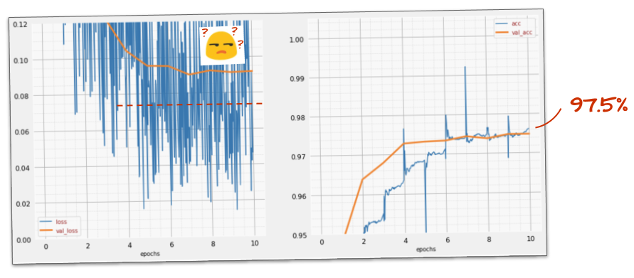
Deeper Roots of Overfitting: The Nature of the Problem

Overfitting isn’t always easily fixed by dropout alone; it stems from fundamental issues.

1. “Too Many Degrees of Freedom”:

• If a network is too large for the complexity of the data, it can simply “memorize” training examples.
• It fails to extract underlying patterns, resulting in poor generalization.

Analogy for ECE:

• Imagine fitting a 10th-order polynomial to only three data points. It will perfectly hit those points but be wild everywhere else.

2. Insufficient Training Data:

• Neural networks are data-hungry.
• With too little data, even a reasonably sized network can overfit because there isn’t enough variety to learn robust patterns.

3. Inadequate Network Architecture:

• Sometimes, the chosen network type isn’t suitable for the data’s structure.
• Our current Dense (fully-connected) only network struggles with image spatial relationships.

While dropout is a great tool, it’s essential to understand that overfitting has deeper, more fundamental causes. Simply applying dropout might not fully solve the problem if these underlying issues are present.

1. Too Many Degrees of Freedom: This happens when your neural network is disproportionately complex for the problem it’s trying to solve. If a network has an excessive number of neurons and parameters, it gains the capacity to essentially memorize the training data points rather than learning the generalized rules that govern them. It’s like fitting a very high-degree polynomial to a small number of data points; it will pass through all of them perfectly (low training loss) but will be wildly inaccurate for any new point. A well-designed network needs a kind of constraint that forces it to extract meaningful, generalizable features.

2. Insufficient Training Data: Deep neural networks are notoriously data-hungry. If you don’t have enough diverse training examples, even a moderately sized network can easily overfit. It simply doesn’t have enough varied information to learn robust patterns that apply broadly. This is a common bottleneck in deploying machine learning in many specialized ECE domains where data acquisition can be costly or difficult.

3. Inadequate Network Architecture: This is a crucial point for our current MNIST task. Recall that we flattened our 28x28 images into a 784-element vector. In doing so, we completely discarded all spatial information – the fact that pixels are arranged in a grid and that neighboring pixels are highly correlated. Our dense network treats every pixel as an independent feature. Handwritten digits, however, are fundamentally made of shapes, edges, and patterns that depend on the spatial arrangement of pixels. A dense network has to “reinvent” this spatial understanding from scratch, which is inefficient and often leads to the performance ceiling we’ve hit.

This inadequacy of our current architecture points us towards the next major advancement for image data: Convolutional Neural Networks (CNNs).

Introduction to Convolutional Neural Networks (CNNs)

Our current model struggles because it treats image pixels as independent features, losing spatial context. Convolutional Neural Networks (CNNs) are designed to leverage this spatial information.

Key Idea:

• Instead of fully-connected layers, CNNs use convolutional filters (kernels).
• These filters slide across the input image, detecting local features like edges, corners, and textures.
• They preserve the spatial relationships between pixels.

Benefits for ECE (Image Processing):

• Feature Hierarchy: Learn increasingly complex features (edges -> shapes -> object parts).
• Parameter Sharing: Detect the same feature anywhere in the image with the same filter.
• Translation Invariance: Robust to slight shifts in object position.
• Crucial for applications like object detection, medical imaging, and autonomous systems.

Important

We’ve hit a performance ceiling with our dense network because it fundamentally misunderstands image data. CNNs are the game-changer here!