Machine Learning

1.6 Neural Networks Part 2: Setting up the Data and the Loss

Imron Rosyadi

Understanding Neural Networks: From Neurons to Layers

Sources

Stanford University CS231n: Deep Learning for Computer Vision

CS231n Deep Learning for Computer Vision

Table of Contents

1. Quick Intro: Linear vs NN
2. Modeling One Neuron
   • Biological Motivation
   • Single Neuron as Linear Classifier
   • Activation Functions
3. Neural Network Architectures
   • Layer-wise Organization
   • Feed-Forward Computation
   • Representational Power
   • Setting Layers & Sizes
4. Summary P1

Table of Contents (Continued)

5. Setting up the Data and Model
   • Data Preprocessing
   • Weight Initialization
   • Batch Normalization
   • Regularization
6. Loss Functions
7. Summary P2
8. Additional References

5. Setting up the Data and the Model

Having introduced the basic neuron model and neural network architectures, we now delve into practical considerations for setting up a robust machine learning system.

These include:

• Data Preprocessing: Preparing input data for optimal network performance.
• Weight Initialization: Setting initial values for network parameters.
• Batch Normalization: Stabilizing and accelerating training.
• Regularization: Techniques to prevent overfitting.

Note

A Neural Network performs a sequence of linear mappings with interwoven non-linearities. These design choices significantly impact training stability and final model performance.

In the first part of this lecture, we established the fundamental building blocks of neural networks: the neuron, activation functions, and how neurons arrange into layers to form an architecture. Now, we shift our focus to the practical steps needed before we even begin the iterative training process.

The choices we make in data preprocessing, how we initialize weights, whether we use techniques like batch normalization, and applying regularization are not just minor details—they are critical engineering decisions that directly influence how quickly and effectively our network learns, and how well it generalizes to new, unseen data. Each of these steps plays a vital role in taking a theoretical model from concept to a high-performing solution.

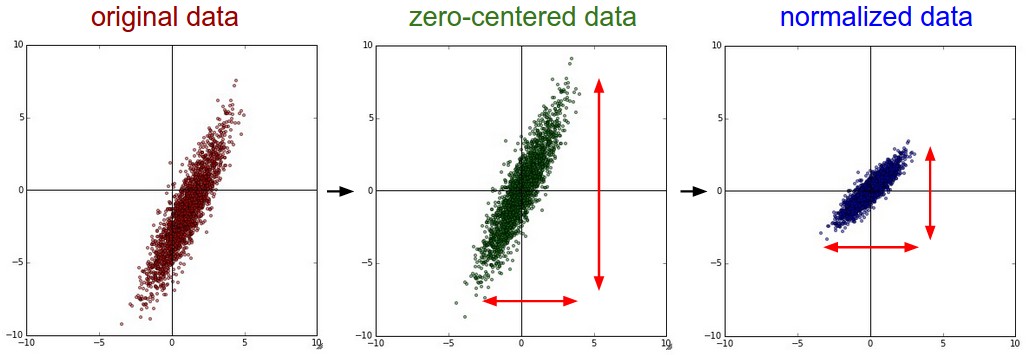
5.1 Data Preprocessing: Centering and Scaling

Three common forms of data preprocessing for a data matrix X of size [N x D] (N data, D dimensions).

1. Mean Subtraction

• Most common form; centers data around the origin.
• X -= np.mean(X, axis = 0) (subtract mean of each feature).
• For images, can subtract global mean or per-channel mean.

2. Normalization

• Scales data dimensions to approximately same range.
• Standardization: Divide by standard deviation after mean-centering: X /= np.std(X, axis = 0).
• Min-Max Scaling: Normalize to range [-1, 1].
• Useful when features have different scales but similar importance.

Left: Original data. Middle: Zero-centered. Right: Scaled by standard deviation.

Important

Pitfall: Preprocessing statistics must be computed only on training data and then applied to validation/test sets to avoid data leakage.

Data preprocessing is a crucial first step. Imagine you have a dataset where one feature, like ‘age’, ranges from 0-100, and another feature, ‘income’, ranges from 0-1,000,000. If we feed these directly into a neural network, the income feature might disproportionately influence the weights and gradients simply because its numerical values are much larger.

Mean subtraction removes the average value from each feature, effectively centering the data around zero. This is geometrically equivalent to shifting the cloud of data points so its center aligns with the origin. Normalization then scales these features. Standardization, by dividing by the standard deviation, results in features with unit variance. This ensures that all features contribute roughly equally to the learning process, regardless of their original scale.

The image helps visualize these steps. The “Common pitfall” is extremely important: to prevent “data leakage” (where information from your test set inadvertently influences the training process), any statistics (like means or standard deviations) used for preprocessing must be calculated only from the training data. These calculated statistics are then used uniformly across the training, validation, and test datasets.

Interactive Data Preprocessing

Observe the effect of mean subtraction and normalization on a small dataset. Modify the data array and rerun the code.

This interactive block allows you to directly manipulate a small data array and see the immediate effects of mean subtraction and standardization.

First, observe the Original Data. Note the different scales of the features (e.g., column 1 vs. column 2). After Mean Subtracted Data, you’ll see that the values are now centered around zero for each feature. The np.mean(data_centered, axis=0) call will show values very close to zero, validating the centering. Finally, the Standardized Data will have features with values typically ranging around -1 to 1, with means near zero and standard deviations near one. This ensures all features are on a comparable scale, preventing one feature from dominating the learning process purely due to its magnitude. Feel free to change the data array to include different values or even columns of constant values to see how the standardization handles them (e.g., if a feature has zero variance, it will be untouched or handled by the std_data[std_data == 0] = 1 line).

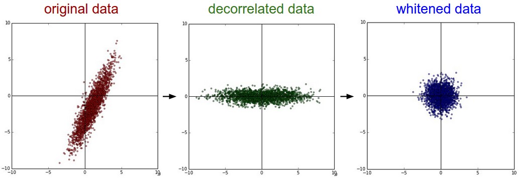
5.1 Data Preprocessing: PCA and Whitening

Advanced preprocessing techniques for decorrelation and isotropic representation.

1. Zero-center the data.
2. Compute the covariance matrix: cov = np.dot(X.T, X) / X.shape[0].
   • Reveals feature correlations.
3. Perform Singular Value Decomposition (SVD) on cov: U,S,V = np.linalg.svd(cov).
   • U: Eigenvectors (new orthogonal basis).
   • S: Singular values (related to variance along new axes).
4. Decorrelate (PCA): Project data onto eigenbasis: Xrot = np.dot(X, U).
   • Xrot_reduced = np.dot(X, U[:,:k]): PCA dimensionality reduction, keeping k most variant dimensions.
5. Whitening: Scale decorrelated data by eigenvalues: Xwhite = Xrot / np.sqrt(S + 1e-5).
   • Transforms data to have zero mean and identity covariance matrix (isotropic Gaussian blob).

Warning

Whitening can exaggerate noise by scaling up low-variance dimensions. A small constant 1e-5 prevents division by zero.

Visualizing PCA/Whitening Transformations

<b>Left</b>: Original toy 2D data.
<b>Middle</b>: After PCA, data is zero-centered and rotated to its eigenbasis (decorrelated).
<b>Right</b>: After Whitening, data dimensions are scaled to unit variance, making it an isotropic Gaussian blob.

Tip

In practice: PCA/Whitening are less common for Convolutional Networks. However, zero-centering is always crucially important, and normalization (dividing by pixel range or standard deviation) is common for images.

PCA and Whitening are more advanced preprocessing steps often used in classical machine learning or for specific types of data. The image shows a beautiful geometric intuition behind these transformations.

After zero-centering, PCA works by rotating the data. The new axes are the “principal components” that capture the most variance in the data. This effectively decorrelates the features. We can also use PCA for dimensionality reduction by keeping only the k principal components that explain most of the variance.

Whitening takes this a step further by scaling each of these decorrelated dimensions so that they all have unit variance. Geometrically, this transforms the data cloud into a spherical (isotropic) Gaussian distribution.

While powerful, these methods are computationally more intensive and generally not directly applied to raw images in modern Convolutional Neural Networks. For CNNs, zero-centering and simple scaling (e.g., dividing pixel values by 255 or subtracting channel means and dividing by channel standard deviations) are typically sufficient and more robust. The caution about Whitening exaggerating noise is also important, as it scales up even the smallest variances.

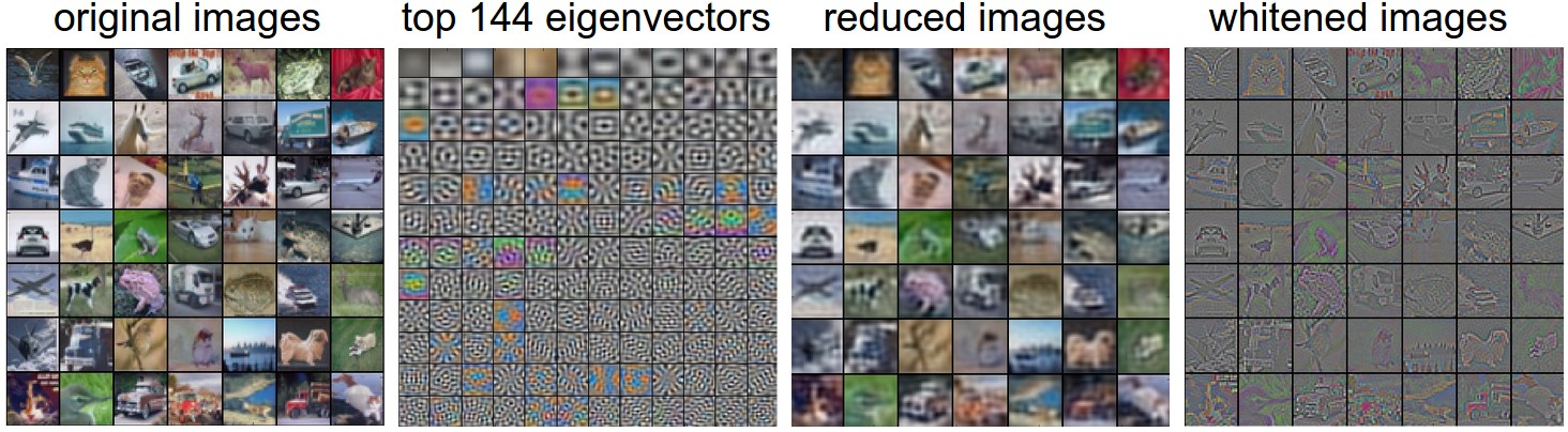
PCA Visualization with CIFAR-10 Features

These visualizations demonstrate PCA’s effect on image features, reducing dimensionality while preserving information.

<b>Left:</b> Sample CIFAR-10 images.
<b>2nd Left:</b> Top 144 eigenvectors (basis images); capture lower frequencies.
<b>2nd Right:</b> Images reconstructed from 144 PCA-reduced features (slightly blurrier, but preserved).
<b>Right:</b> Whitened images; higher frequencies exaggerated.

This slide offers a qualitative understanding of PCA in the context of image data, specifically CIFAR-10. If we treat each image as a high-dimensional vector, we can apply PCA. The “eigenvectors” in this context can be visualized as synthetic images themselves. The top eigenvectors (second from left) represent dominant patterns or lower frequencies in the dataset.

When we reduce an image to its top 144 PCA components and then reconstruct it (second from right), you can see that despite using significantly fewer numbers (144 vs 3072), much of the visual information—the general shape and color—is retained, although some fine details (higher frequencies) are lost, resulting in blurriness.

The rightmost image, showing the “whitened” representation, further illustrates the impact of scaling by eigenvalues. Here, the low-frequency components, which naturally have high variance in images, are compressed, while the higher-frequency, often noisy components are amplified. This leads to a distinct, “edge-enhanced” appearance, which can be useful in some contexts but often problematic for noise sensitivity. This helps illustrate why simple normalization is preferred for CNNs in practice.

5.2 Weight Initialization

Crucial for network stability and convergence. Poor initialization can lead to vanishing/exploding gradients or slow learning.

Pitfall: All Zero Initialization

• W = np.zeros((D, H))
• Problem: Every neuron computes the same output, gradients, and updates.
• Leads to a symmetric network where all neurons learn the same features.
• Result: No symmetry breaking, network effectively becomes a single neuron per layer.

Small Random Numbers (Symmetry Breaking)

• W = 0.01 * np.random.randn(D, H)
• Initialize weights to small, random values (e.g., from a Gaussian distribution).
• Neurons start unique, compute distinct updates, and break symmetry.

Warning

Very small weights can lead to very small gradients during backpropagation, diminishing the “gradient signal” in deep networks.

Weight initialization is far more important than it might seem at first glance. It sets the starting point for the optimization process, and a bad start can either prevent the network from learning anything or significantly slow down its convergence.

The “all zero initialization” is a classic example of what not to do. If all weights are zero, then every neuron in a given layer will produce the same output, and during backpropagation, they will all receive the identical gradients. This means they will all update their weights identically, and effectively become indistinguishable, failing to learn diverse features.

The simplest solution is to initialize with “small random numbers.” This breaks the symmetry, ensuring that each neuron starts in a unique state and thus learns different features. However, even this has a caveat: if values are too small, the gradients flowing back through the network can become very tiny, leading to the vanishing gradient problem, especially in deeper networks. This highlights a balancing act we need to achieve: not too uniform, not too small, and preferably calibrated.

5.2 Weight Initialization: Calibrating Variances

Problem: Variance of a neuron’s output grows with the number of inputs (n).

Proposed Solution: Scale initial weights by 1/sqrt(n) to normalize output variance.

Heuristic: w = np.random.randn(n) / np.sqrt(n)

• Ensures all neurons initially have approximately the same output distribution.
• Empirically improves convergence rate.

Derivation Sketch:

For a neuron’s raw activation s = _i^n w_i x_i with zero-mean inputs/weights: \[ \text{Var}(s) = \left( n \text{Var}(w) \right) \text{Var}(x) \]

To make \(\text{Var}(s) \approx \text{Var}(x)\), we need \(n \text{Var}(w) = 1\), so \(\text{Var}(w) = 1/n\).

If \(w_i \sim N(0, \sigma^2)\), then \(\sigma^2 = 1/n\), so \(\sigma = 1/\sqrt{n}\).

Tip

Current Recommendation (He et al. 2015): For ReLU neurons, use \(\text{Var}(w) = 2/n\). Thus, w = np.random.randn(n) * np.sqrt(2.0/n).

A significant challenge with random initialization is that the variance of a neuron’s output can increase with the number of its inputs (n). If outputs get too large, they can cause activation functions (like sigmoid or tanh) to saturate, leading to vanishing gradients. If they’re too small, gradients also vanish.

The solution is to “calibrate” the variance. The core idea is to scale the initial weights such that the variance of the neuron’s output remains stable across layers, ideally similar to the variance of its inputs. The derivation shows how 1/sqrt(n) comes about.

For ReLU activation functions, which are very common, a slightly different scaling factor was derived by He et al. (2015), pushing the variance to 2/n, leading to the np.sqrt(2.0/n) scaling factor. This initialization is widely used and highly recommended for networks employing ReLU. This helps maintain healthy gradients throughout training.

Interactive Weight Initialization Variance

Observe how weight scaling affects the variance of a neuron’s output.

Adjust the number_of_inputs and scaling_factor to see their impact.

viewof number_of_inputs = Inputs.range([1, 100], {value: 50, step: 1, label: "Number of Inputs (n)"});
viewof scaling_factor_val = Inputs.range([0.01, 2.0], {value: 1.0, step: 0.01, label: "Weight Scaling Factor"});

This interactive example allows you to explore the relationship between the number of inputs to a neuron (n) and the scaling of its initial weights on the variance of its output s.

• number_of_inputs (n): Represents the “fan-in” to the neuron.
• scaling_factor_val: This explicitly controls the sigma used to initialize the weights.

Observe how Variance of neuron output (s) changes. If scaling_factor_val is 1.0 (default for np.random.randn), try increasing n. You’ll see var_s increase proportionally to n. This illustrates the problem: a deeper network with many inputs per neuron would quickly lead to very large outputs.

Now, try to manually set scaling_factor_val to 1/sqrt(n) or sqrt(2/n) (where n is your current number_of_inputs) and observe if var_s approaches 1.0 or 2.0 respectively (reflecting Var(x) if Var(x)=1). For instance, if n=50, try 1/sqrt(50) (approx 0.14) or sqrt(2/50) (approx 0.2). You should see the variance stabilize.

This demonstrates why proper scaling is critical for maintaining healthy signal magnitudes throughout the network, preventing activations from exploding or vanishing and facilitating stable training.

5.2 Weight Initialization: Other Considerations

• Sparse Initialization:
  • Set all weight matrices to zero, but randomly connect a fixed, small number of neurons (e.g., 10) with small Gaussian weights.
  • Addresses uncalibrated variance but less common than He/Xavier.
• Initializing Biases:
  • Usually initialized to zero. Symmetry breaking is handled by weights.
  • For ReLU, sometimes a small constant (e.g., 0.01) is used to ensure units fire initially, but this is not consistently beneficial.

Tip

In practice: Current recommendation for ReLU is w = np.random.randn(n) * np.sqrt(2.0/n). Biases are typically initialized to zero.

5.3 Batch Normalization (BatchNorm)

A technique to stabilize and accelerate deep network training.

Core Idea:

Explicitly forces activations throughout the network to take on a unit Gaussian distribution at the beginning of training for each mini-batch.

Mechanism:

For each feature map in a layer, normalize its activations:

1. Calculate mean \(\mu_B\) and variance \(\sigma_B^2\) for the current mini-batch B.
2. Normalize: \(\hat{x}_i = (x_i - \mu_B) / \sqrt{\sigma_B^2 + \epsilon}\)
3. Scale and Shift: \(y_i = \gamma \hat{x}_i + \beta\)
   • \(\gamma, \beta\) are learnable parameters (scale and shift).
   • Allows network to restore original distribution if optimal.

Important

Insert the BatchNorm layer immediately after fully connected/convolutional layers and before non-linearities.

Visualizing Batch Normalization’s Placement

graph TD
    Input --> FC_Layer(Fully Connected Layer)
    FC_Layer --> BatchNorm_Layer(Batch Normalization Layer)
    BatchNorm_Layer --> Activation_Function("Activation Function (e.g., ReLU)")
    Activation_Function --> Next_Layer(...)

    style Input fill:#e0f7fa,stroke:#333,stroke-width:2px;
    style FC_Layer fill:#fff8e1,stroke:#333,stroke-width:2px;
    style BatchNorm_Layer fill:#e8f5e9,stroke:#333,stroke-width:2px;
    style Activation_Function fill:#ffebee,stroke:#333,stroke-width:2px;
    style Next_Layer fill:#e0f7fa,stroke:#333,stroke-width:2px;

Benefits of BatchNorm:

• Greatly improves training speed.
• Makes networks significantly more robust to bad initialization.
• Acts as a form of regularization, reducing reliance on other techniques like Dropout.
• Allows for higher learning rates.

Batch Normalization, introduced by Ioffe and Szegedy in 2015, is a major breakthrough in deep learning training. It addresses the “internal covariate shift” problem, where the distribution of activations changes throughout training as parameters in previous layers update. This constant shifting makes it difficult for deeper layers to learn effective representations.

The core idea is simple: for each mini-batch during training, normalize the activations of each feature to have zero mean and unit variance. This is done on a per-feature basis. However, simply normalizing might restrict the network’s representational power. To counteract this, BatchNorm introduces two learnable parameters, gamma (scale) and beta (shift), which allow the network to optimally re-scale and re-shift the normalized values. If it’s optimal for a layer to have a different mean or variance, the network can learn to restore that.

The Mermaid diagram clearly shows BatchNorm’s preferred placement: always after the linear transformation (FC or Conv layer) and before the non-linear activation function. This ensures that the inputs to the non-linearity are always in a stable, well-behaved range. The benefits are profound, leading to faster training, better robustness, and often improved generalization.

5.4 Regularization: Preventing Overfitting

Techniques to control network capacity and improve generalization to unseen data.

L2 Regularization (Weight Decay)

• Most common form.
• Adds \(\frac{1}{2}\lambda w^2\) to the objective for each weight \(w\).
• Intuition: Penalizes large weights, preferring diffuse weight vectors.
• Encourages the network to use all inputs a little, rather than some inputs a lot.
• During gradient descent, causes weights to decay linearly towards zero: W += -lambda * W.

L1 Regularization

• Adds \(\lambda \mid w \mid\) to the objective for each weight w.
• Property: Leads to sparse weight vectors (many weights become exactly zero).
• Useful for feature selection; neurons rely on a sparse subset of inputs.
• Can be combined with L2: Elastic Net Regularization.

Note

L2 regularization generally gives superior performance unless explicit feature selection (sparsity) is desired.

5.4 Regularization: Max Norm & Dropout

Max Norm Constraints

• Enforces an absolute upper bound on the magnitude of each neuron’s weight vector.
• Weight vector \(\vec{w}\) is clamped to satisfy \(\Vert \vec{w} \Vert_2 < c\) after each update (e.g., \(c=3\) or \(4\)).
• Benefit: Prevents “exploding” network activations, even with high learning rates.

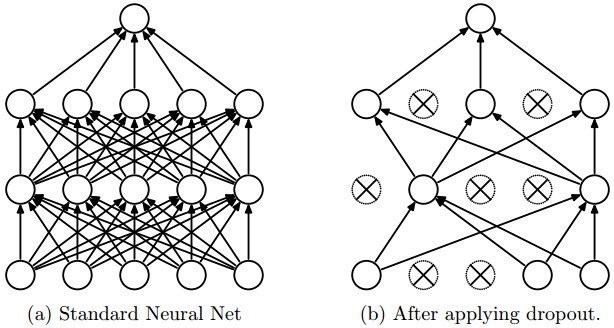
Dropout

• Extremely effective and simple regularization technique.
• During training, each neuron is kept active with probability \(p\) (hyperparameter, e.g., 0.5) or set to zero otherwise.

Dropout can be seen as training an ensemble of neural networks.

Important

Dropout, L2, L1, and Max Norm address different aspects of overfitting and can often be combined effectively.

Dropout: Implementation

Vanilla Dropout (Not Recommended)

Scales activations at test time.

p = 0.5 # probability of keeping a unit active

def train_step(X):
  H1 = np.maximum(0, np.dot(W1, X) + b1)
  U1 = np.random.rand(*H1.shape) < p # binary mask
  H1 *= U1 # drop!
  # ... second layer ...

def predict(X):
  H1 = np.maximum(0, np.dot(W1, X) + b1) * p # NOTE: scale by p
  # ... second layer ...

Dropout: Implementation

Inverted Dropout (Recommended)

Scales activations at train time, leaving test time untouched.

p = 0.5 # probability of keeping a unit active

def train_step(X):
  H1 = np.maximum(0, np.dot(W1, X) + b1)
  U1 = (np.random.rand(*H1.shape) < p) / p # NOTE: scale by 1/p
  H1 *= U1 # drop!
  # ... second layer ...

def predict(X):
  H1 = np.maximum(0, np.dot(W1, X) + b1) # NO scaling needed
  # ... second layer ...

Tip

In practice: Use a single, global L2 regularization strength (cross-validated) with inverted dropout (p=0.5 is a good default).

Dropout is an ingenious and remarkably simple regularization technique. During training, it randomly “turns off” (sets to zero) a fraction of neurons in a layer. This forces the network to learn more robust features because no single neuron can rely too heavily on the presence of another. It prevents complex co-adaptations and effectively trains an “ensemble” of many smaller networks.

The crucial detail is how it’s handled during prediction. To maintain the same expected output magnitude as during training, we usually have to scale the activations. “Vanilla Dropout” scales at test time, which can complicate deployment. “Inverted Dropout,” the recommended approach, performs this scaling during training (by dividing by p), so that at test time, no modifications are needed. This makes the prediction code cleaner and more efficient.

The figure illustrates dropout as sampling a sub-network from the full network. The “In practice” tip is a strong guide for initial experiments: combine L2 regularization with inverted dropout.

Interactive Dropout Simulation

Simulate inverted dropout on a small matrix. Adjust dropout_probability_p to see how many elements are dropped and scaled.

viewof dropout_probability_p = Inputs.range([0.1, 1.0], {value: 0.5, step: 0.1, label: "Dropout Probability (p)"});

This Pyodide block provides a hands-on demonstration of Inverted Dropout. You can see how:

1. A random random_mask is generated based on the dropout_probability_p. Elements are True (kept) with probability p, and False (dropped) with probability 1-p.
2. The mask U is created by dividing the random_mask by p. This 1/p scaling is the core of inverted dropout, ensuring that the expected sum of activations remains the same after dropout.
3. The H_original activations are then multiplied by U to get H_dropped_scaled. Notice how some values become zero (dropped), and the values that are kept are scaled up by 1/p.

Experiment by changing the dropout_probability_p:

• A p=1.0 means no dropout; all elements are kept and scaled by 1/1.0 = 1, so H_dropped_scaled should be identical to H_original.
• A smaller p (e.g., 0.1) will result in more elements being dropped and the kept elements being scaled up by a larger factor (e.g., 1/0.1 = 10).

This interactive visualization helps solidify the understanding of how inverted dropout operates and why the scaling factor 1/p is essential.

6. Loss Functions

The “data loss” component of your objective function. Measures compatibility between prediction (f) and ground truth label (y). Total loss: \(L = \frac{1}{N} \sum_i L_i + \text{Regularization Loss}\).

6.1 Classification

One correct label \(y_i\) from a fixed set.

• SVM Loss (Weston Watkins): \[L_i = \sum_{j\neq y_i} \max(0, f_j - f_{y_i} + 1)\]
  • Also common: squared hinge loss \(\max(0, f_j - f_{y_i} + 1)^2\).
• Softmax Loss (Cross-Entropy): \[L_i = -\log\left(\frac{e^{f_{y_i}}}{ \sum_j e^{f_j} }\right)\]
  • Interprets scores \(f_j\) as unnormalized log-probabilities.

Note

Large Number of Classes Problem: For huge label sets (e.g., ImageNet 22k, NLP vocabularies), computing full Softmax is expensive. Solutions like Hierarchical Softmax approximate by structuring labels in a tree.

Loss functions are fundamental in supervised learning; they quantify how “wrong” our model’s predictions are. The goal of training is to minimize this loss, along with the regularization loss discussed earlier.

For classification, where each example has one correct label, two major loss functions stand out. The SVM loss aims to ensure that the score of the correct class is at least a certain margin (typically 1) higher than the scores of all incorrect classes. If this margin is not met, a penalty is incurred.

The Softmax loss, also known as cross-entropy loss, is perhaps more intuitive. It transforms the raw scores into probabilities using the softmax function and then penalizes the model based on the (negative) log-probability assigned to the true class. The higher the probability of the correct class, the lower the loss.

When you have thousands or even millions of classes (like in large language models or image datasets with very fine-grained categories), computing the sum over all possible classes in Softmax can become computationally prohibitive. Hierarchical Softmax is one technique that tries to mitigate this by creating a tree structure for classes, where decisions are made at each node, dramatically reducing the number of computations.

Interactive Classification Loss Plot

Compare SVM and Softmax loss for a single example prediction. Adjust the correct_class_score and incorrect_class_score to see their impact on loss.

viewof correct_score = Inputs.range([-3, 5], {value: 2, step: 0.1, label: "Score for Correct Class"});
viewof incorrect_score = Inputs.range([-3, 5], {value: 0.5, step: 0.1, label: "Score for Incorrect Class"});

This interactive plot helps compare the behavior of SVM and Softmax loss functions. We simulate a scenario with two classes, where one is correct and the other is incorrect.

• X-axis: Represents the score assigned by the model to the incorrect class.
• Y-axis: Represents the resulting loss.
• The correct_class_score slider allows you to fix the score of the correct class.

Observations:

• SVM Loss (Blue): Notice that when the incorrect class score is much lower than the correct class score (by at least the margin of 1), the SVM loss becomes 0. This means the SVM is “satisfied” and no longer penalizes the model. It cares only about achieving this margin.
• Softmax Loss (Red): The Softmax loss never reaches 0, even when the incorrect score is very low. It continuously encourages the correct class score to be as high as possible and incorrect class scores to be as low as possible, pushing towards an ideal probability of 1 for the correct class.

Adjust the sliders to explore different scenarios. For instance, make the incorrect_class_score higher than correct_class_score to see how both losses increase. This demonstrates their distinct behaviors in guiding the optimization process. SVM creates a “flat” loss landscape once the margin is met, while Softmax always provides a gradient to improve probabilities.

6.2 Attribute Classification

Attribute Classification

• For multi-label problems where an example can have multiple non-exclusive attributes (e.g., an image with multiple hashtags).
• Approach: Build a binary classifier for each attribute independently.
• SVM-like Loss: \[L_i = \sum_j \max(0, 1 - y_{ij} f_j)\]
  • \(y_{ij} \in \{+1, -1\}\), \(f_j\) is the score for attribute \(j\).
• Logistic Regression Loss: \[L_i = -\sum_j y_{ij} \log(\sigma(f_j)) + (1 - y_{ij}) \log(1 - \sigma(f_j))\]
  • \(y_{ij} \in \{0, 1\}\), \(\sigma(\cdot)\) is the sigmoid function.

6.3 Regression

Regression (Predicting Real-Valued Quantities)

• Commonly uses L2 or L1 norm of the difference.
• L2 Loss (Squared Error): \[L_i = \Vert f - y_i \Vert_2^2\]
• L1 Loss (Absolute Error): \[L_i = \Vert f - y_i \Vert_1 = \sum_j \mid f_j - (y_i)_j \mid\]

Warning

L2 loss is much harder to optimize and less robust to outliers than Softmax. Consider quantizing outputs into bins and performing classification whenever possible for regression tasks.

Beyond single-label classification, we encounter other types of problems. Attribute classification, also known as multi-label classification, is when an instance can belong to multiple categories simultaneously (e.g., an image of a dog and a cat). The most common approach is to treat each attribute as an independent binary classification problem, applying either an SVM-like hinge loss or a logistic regression (binary cross-entropy) loss to each attribute’s score.

Regression, on the other hand, deals with predicting continuous, real-valued quantities. The L2 (squared error) and L1 (absolute error) norms are the standard choices. L2 loss is differentiable everywhere and heavily penalizes large errors, pushing the model to be very accurate for all points. However, this also makes it sensitive to outliers. L1 loss is more robust to outliers as it scales linearly with the error.

Critically, the warning reminds us that L2 loss can be very fragile. Neural networks might struggle to output exact values. It is often a strong engineering heuristic to convert a regression problem into a classification problem by discretizing the output range into bins. For example, predicting house prices might become classifying into “price range” bins. This approach can be more stable and provide confidence estimates over the predicted range.

7. Summary (Part 2)

• Data Preprocessing: Crucial for model stability and performance.
  • Always zero-center data.
  • Normalize data scale (e.g., by standard deviation).
  • Compute preprocessing statistics only on training data.
• Weight Initialization:
  • Avoid zero initialization; use small random numbers.
  • Recommended for ReLU: w = np.random.randn(n) * np.sqrt(2.0/n).
  • Biases typically initialized to zero.
• Batch Normalization:
  • Stabilizes training and speeds up convergence.
  • Insert after FC/Conv layers, before non-linearities.
  • Makes networks robust to poor initialization.
• Regularization: Prevents overfitting.
  • Commonly use L2 regularization and inverted Dropout (p=0.5 is a good default).
• Loss Functions:
  • Classification: SVM loss, Softmax (Cross-entropy) loss.
  • Attribute Classification: Per-attribute binary classifiers (SVM-like or Logistic Regression).
  • Regression: L2 or L1 Loss. Prefer classification for regression when possible.