Machine Learning

1.5 Neural Networks Part 1: Setting up the Architecture

Imron Rosyadi

Understanding Neural Networks: From Neurons to Layers

Sources

Stanford University CS231n: Deep Learning for Computer Vision

CS231n Deep Learning for Computer Vision

Table of Contents

1. Quick Intro: Linear vs NN
2. Modeling One Neuron
   • Biological Motivation
   • Single Neuron as Linear Classifier
   • Activation Functions
3. Neural Network Architectures
   • Layer-wise Organization
   • Feed-Forward Computation
   • Representational Power
   • Setting Layers & Sizes
4. Summary
5. Additional References

1. Quick Intro: Beyond Linear Models

Linear Classification:

• Scores obtained directly from weighted input sum.
• Example: \( s = W x \)
  • \(x\): input vector (e.g., image pixels).
  • \(W\): weight matrix.
  • \(s\): class scores.

Note

Issue: Limited to linear decision boundaries.

Neural Network Approach (2-layer):

• Introduces a non-linear transformation.
• Example: \( s = W_2 (0, W_1 x) \)
  • \(W_1\): First layer weights.
  • \((0, )\): Element-wise non-linearity (ReLU).
  • \(W_2\): Second layer weights.

Important

The non-linearity is crucial for modeling complex relationships and introducing the “wiggle”.

In traditional linear classification, like SVMs or Softmax, we directly compute scores as a linear combination of inputs and weights. For example, for an image classification task, say CIFAR-10, an input image x (3072 pixels) is multiplied by a weight matrix W (10x3072) to produce 10 class scores. This approach is simple and interpretable but inherently limited to “linear” decision boundaries.

Neural networks overcome this by introducing non-linear activation functions between layers. A simple two-layer network, as shown in the example s = W2 max(0, W1 x), first transforms the input x using W1, then applies a non-linear function (here, max(0,.) which is ReLU), and finally transforms it again with W2 to get the scores. This non-linearity is the key component; without it, multiple linear layers would collapse into a single linear operation, offering no additional power beyond a simple linear classifier. This “wiggle” allows neural networks to learn intricate, non-linear patterns in data.

Quick Intro: Visualizing the Flow

graph LR
    Input["Input Image (x)"] --> W1_Layer("Layer 1 - W1")
    W1_Layer --> Nonlinearity["Non-Linear Activation (max(0, .))"]
    Nonlinearity --> W2_Layer("Layer 2 - W2")
    W2_Layer --> Scores["Output Scores (s)"]

    style Input fill:#f9f,stroke:#333,stroke-width:2px;
    style Scores fill:#bbf,stroke:#333,stroke-width:2px;

• Deeper Networks:
  • A three-layer network: \( s = W_3 (0, W_2 (0, W_1 x)) \)
  • Adds more non-linear transformations.
  • Parameters \(W_i\) are learned via stochastic gradient descent and backpropagation.

This flowchart illustrates the forward pass of the two-layer neural network we just discussed. The input image x first goes through a linear transformation by W1. The result then undergoes a non-linear activation, which introduces the capacity to learn complex, non-linear relationships. Finally, another linear transformation by W2 produces the output class scores s.

For deeper networks, this process simply stacks more such layers, each with its own weights and non-linear activation. The key takeaway is that each layer adds a level of abstraction and complexity, allowing the network to learn rich representations of the input data. The learning process involves adjusting all these weight matrices, W1, W2, W3, based on the error in the output, using algorithms like backpropagation.

2. Modeling One Neuron: Biological Motivation

Biological Neuron (Left):

• Dendrites: Receive input signals.
• Cell Body: Integrates signals.
• Axon: Transmits output signals.
• Synapses: Connections to other neurons, with variable strengths.

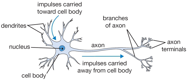
A cartoon drawing of a biological neuron.

Computational Model (Right):

• Inputs (\(x_i\)) correspond to signals from other neurons.
• Weights (\(w_i\)) represent synaptic strengths (learnable).
• Summation: \(_i w_i x_i + b\) (cell body processing).
• Activation function (\(f\)): Simulates firing rate.

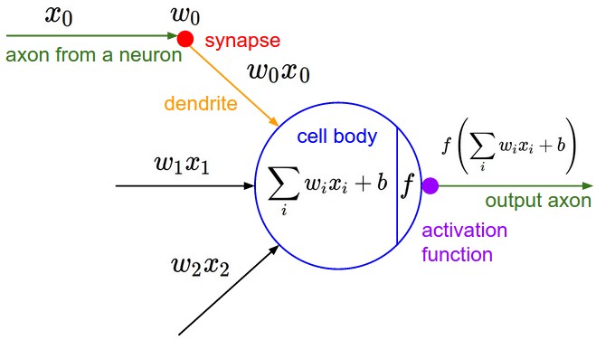
Mathematical model of a neuron.

The concept of a neural network is loosely inspired by biological neurons. On the left, you see a simplified diagram of a biological neuron. It receives signals through dendrites, processes them in the cell body, and sends out signals through its axon, which connects to other neurons via synapses.

On the right, we have the mathematical model. Each input x_i is multiplied by a corresponding weight w_i, mimicking synaptic strength. These weighted inputs are summed, along with a bias term b, representing the cell body’s integration. Finally, an activation function f (like sigmoid here) is applied to this sum. This function models the neuron’s “firing rate,” squashing the output to a specific range (e.g., 0 to 1). The weights w_i and bias b are the learnable parameters in this computational model.

It’s important to remember that this is a highly simplified model. Biological neurons are far more complex, with dynamic, non-linear dendritic computations and precise spike timing. We abstract away much of this complexity for computational tractability and effective machine learning.

Modeling One Neuron: Interactive Forward Pass

Let’s simulate a single neuron’s forward computation. You can modify inputs, weights, and bias to observe the firing_rate.

This interactive code block demonstrates the forward pass of our single neuron model. The sigmoid function is defined as our activation function. You are encouraged to change the values of inputs, weights, and bias within the designated section.

Observe how changes to these parameters affect the cell_body_sum and subsequently the final firing_rate. For instance, try making the weights larger, smaller, or even negative, and see how the neuron’s output responds to different input patterns. This helps build an intuition for how the neuron “reacts” to its inputs based on its learned parameters.

Single Neuron as a Linear Classifier

A single neuron’s output \((_i w_i x_i + b)\) can be interpreted as a probability.

• Binary Softmax Classifier (Logistic Regression)
  • \(P(y=1 x; w) = (_i w_i x_i + b)\)
  • \(P(y=0 x; w) = 1 - P(y=1 x; w)\)
  • Optimized with cross-entropy loss.
• Binary SVM Classifier
  • The neuron’s output can be combined with a max-margin hinge loss.
  • The neuron effectively “fires” if the input falls into one class, and not for the other.

Tip

Regularization: In this context, regularization loss (e.g., L2) can be seen as “gradual forgetting” of synaptic weights.

Note

A single neuron can be used to implement a binary classifier (e.g., binary Softmax or binary SVM classifiers).

This slide highlights the classification capabilities of a single neuron. When combined with a sigmoid activation function, the neuron’s output, ranging from 0 to 1, can be directly interpreted as the probability of an input belonging to one of two classes. This forms the basis of a Binary Softmax classifier, often referred to as logistic regression. The model is trained by minimizing the cross-entropy loss, which measures the difference between predicted and true probabilities.

Alternatively, by attaching a max-margin hinge loss to the neuron’s output, it can be trained to function as a binary Support Vector Machine. In this case, the neuron aims to correctly classify inputs with a maximum margin between the classes.

The beauty of this is that the regularization terms used in these classifiers, like L2 regularization, can be seen from a biological perspective as a mechanism for “gradual forgetting,” naturally driving less important synaptic weights towards zero. This ensures that the model doesn’t become overly reliant on any single input feature, contributing to better generalization.

3. Commonly Used Activation Functions

An activation function (or non-linearity) takes a single number and performs a fixed mathematical operation.

Sigmoid Function \((x) = 1 / (1 + e^{-x})\)

• Squashes real numbers to range [0, 1].
• Historically popular for “firing rate” interpretation.

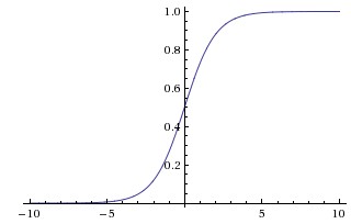
Sigmoid non-linearity.

Warning

Drawbacks:

• Saturates and kills gradients: At tails (0 or 1), gradient is near zero, hindering learning.
• Non-zero-centered output: Can lead to zig-zagging gradient updates.

Tanh Function \((x) = 2 (2x) -1\) * Squashes real numbers to range [-1, 1]. * Zero-centered output - an improvement over sigmoid.

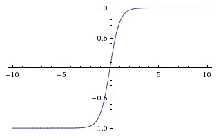
Tanh non-linearity.

Note

Preferred over Sigmoid: Due to its zero-centered output, it generally performs better than sigmoid. Still suffers from saturation.

Activation functions are crucial for introducing non-linearity into neural networks, allowing complex patterns to be learned. Without them, stacking multiple layers would simply result in another linear function, negating the benefits of depth.

The Sigmoid function, while historically significant, has severe limitations. Its “S” shape means that for very large positive or negative inputs, the output saturates quickly, causing its derivative (gradient) to become extremely small. During backpropagation, this small gradient effectively “kills” the learning signal for upstream layers, a problem known as the vanishing gradient problem. Additionally, its output is always positive, which can lead to inefficient “zig-zagging” in gradient descent as weight updates might always be in the same direction.

The Tanh function offers an improvement by being zero-centered, addressing one of sigmoid’s issues. However, it still suffers from the saturation problem, meaning large inputs will still lead to small gradients and hinder learning in those regions. Despite this, Tanh is generally preferred over Sigmoid when choosing classic activation functions.

Activation Functions: ReLU and Variants

Rectified Linear Unit (ReLU) \(f(x) = (0, x)\)

• Output is 0 for negative input, \(x\) for positive input.
• Pros:
  • Accelerates convergence significantly.
  • Computationally efficient (simple thresholding).
  • Does not saturate in the positive region.

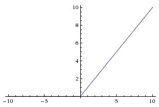
ReLU activation function.

ReLU Cons & Variants:

• “Dying ReLU” problem: Neurons can become inactive (output 0) for all future inputs if gradients are too large.
• Leaky ReLU: \(f(x) = (x < 0) (x) + (x ) (x)\)
  • Introduces a small positive slope \(\) for negative inputs (e.g., 0.01).
  • Aims to prevent dying ReLUs.
• Maxout: \((w_1^Tx+b_1, w_2^Tx + b_2)\)
  • Generalizes ReLU and its leaky version.
  • No saturation, no dying problem.
  • Drawback: Doubles the number of parameters per neuron.

Warning

For ReLU, monitor “dead” units. High learning rates can exacerbate the dying ReLU problem.

ReLU has become the most popular activation function in deep learning. Its simple form, max(0, x), offers significant advantages: it’s computationally very cheap and, crucially, it doesn’t suffer from saturation in the positive region, which greatly accelerates training compared to sigmoid or tanh.

However, ReLU has its own Achilles’ heel: the “dying ReLU” problem. If a neuron’s weights are updated in such a way that its output is always negative for all training examples, the ReLU function will consistently output zero. This means its gradient will also be zero, and the neuron will stop learning completely—it essentially “dies.”

To address this, variants like Leaky ReLU introduce a small, non-zero slope for negative inputs, ensuring that there’s always a gradient flowing through the neuron, even if it’s small. Maxout further generalizes this, offering even better properties but at the cost of increasing the number of parameters, which can make models more prone to overfitting if not properly regularized.

The TLDR for activation functions: Start with ReLU. Be mindful of its potential pitfalls and consider Leaky ReLU or Maxout if you encounter issues like dying neurons or want to push performance further. Avoid sigmoid in hidden layers. Tanh is an option, but generally, ReLU-based activations are preferred.

Interactive Activation Functions

Explore how Sigmoid, Tanh, and ReLU functions respond to different input values. Adjust the Input X Value slider to see the corresponding output for each function.

viewof x_input = Inputs.range([-5, 5], {value: 0, step: 0.1, label: "Input X Value"});

This interactive plot allows you to visually compare the behavior of the three main activation functions: Sigmoid, Tanh, and ReLU. Observe how the output f(x) changes as you move the Input X Value slider.

• Sigmoid (Blue): Notice how it flattens out (saturates) at extreme positive and negative values, leading to very small slopes. Its output is always between 0 and 1.
• Tanh (Red): Similar to Sigmoid, it also saturates, but its output is centered around 0, ranging from -1 to 1.
• ReLU (Green): For positive inputs, it behaves linearly, maintaining a constant slope (gradient of 1). For negative inputs, it’s strictly zero. This linear behavior in the positive region is why it helps accelerate training.

Pay close attention to the gradients (slopes) at different points. The flat regions for Sigmoid and Tanh demonstrate the “vanishing gradient” problem, which ReLU largely avoids in its positive region.

4. Neural Network Architectures

Layer-wise Organization

Neural Networks are collections of neurons connected in an acyclic graph. Most common organizations are into distinct layers.

Fully-Connected Layer:

• Neurons between adjacent layers are fully pairwise connected.
• Neurons within a single layer share no connections.

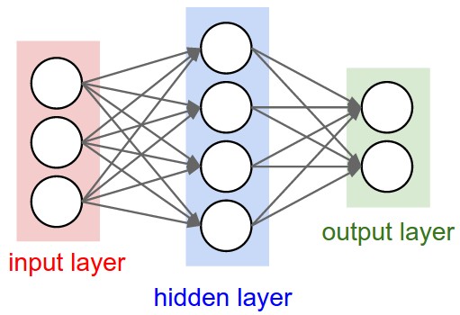
Two-layer Neural Network topology.

Example - 3-Layer Network:

• Three inputs.
• Two hidden layers, each with 4 neurons.
• One output layer.

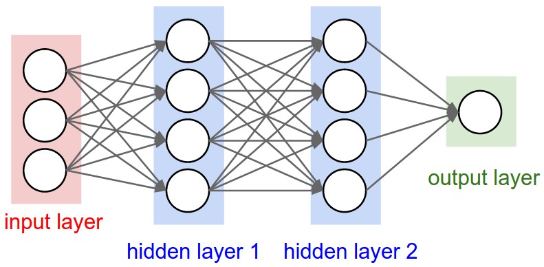
Three-layer Neural Network topology.

Neural networks are structured as layers of interconnected neurons. The key rule is that connections are acyclic, meaning there are no feedback loops that would cause infinite computation in a feedforward network.

The most common layer type in a basic neural network is the “fully-connected” layer. In such a layer, every neuron in one layer sends its output to every neuron in the next layer. However, crucially, neurons within the same layer do not connect to each other. This clear, layered structure makes computation highly efficient, primarily through matrix operations.

The images show classic examples: a 2-layer network with one hidden layer and an output layer, and a 3-layer network with two hidden layers. Notice how each layer builds upon the outputs of the previous one, creating a hierarchical representation of the data.

Neural Network Architecture: A Deeper Look

Let’s visualize the connections in a 3-layer neural network with 3 inputs, two hidden layers of 4 neurons, and 1 output.

This Graphviz diagram provides a more explicit visualization of the connections within a 3-layer fully-connected neural network. You can clearly see the distinct input, hidden (two layers), and output layers.

Each input x0, x1, x2 connected to all neurons in the first hidden layer. Similarly, all neurons in Hidden Layer 1 connect to all neurons in Hidden Layer 2, and all neurons in Hidden Layer 2 connect to the single output neuron. This “all-to-all” connectivity between layers defines a fully-connected architecture. Notice the absence of connections within any given layer, confirming the layered structure. This diagram helps solidify the concept of how information flows through the network.

Naming Conventions & Sizing Neural Networks

• N-layer network: Number of hidden layers + output layer (input layer is not usually counted).
  • Single-layer network: No hidden layers (e.g., Logistic Regression).
  • Artificial Neural Networks (ANN) or Multi-Layer Perceptrons (MLP) are common synonyms.
  • “Units” is a more general term than “neurons”.
• Output Layer: Typically has no activation function (or linear identity) for class scores or regression targets.

Sizing Metrics:

1. Number of neurons (excluding input).
2. Number of parameters (weights + biases) - more common.

Example 1 (2-layer NN):

• 4 hidden, 2 output neurons.
• Weights: \([3 ] + [4 ] = 12 + 8 = 20\)
• Biases: \(4 + 2 = 6\)
• Total Parameters: \(20 + 6 = 26\)

Example 2 (3-layer NN):

• 4 hidden (H1), 4 hidden (H2), 1 output neuron.
• Weights: \([3 ] + [4 ] + [4 ] = 12 + 16 + 4 = 32\)
• Biases: \(4 + 4 + 1 = 9\)
• Total Parameters: \(32 + 9 = 41\)

Tip

Modern Convolutional Networks can have 10-20 layers and >100 million parameters (“deep learning”).

Understanding how to talk about and size neural networks is fundamental. When we refer to an “N-layer neural network,” N typically refers to the number of hidden layers plus the output layer, excluding the input layer. So, a network with just an input and output layer (like logistic regression) is often called a one-layer network.

The most practical way to measure a network’s size is by its total number of learnable parameters, which include all the weights and biases. I’ve broken down the calculation for the two example networks from previous slides. This kind of calculation is crucial for estimating computational requirements and potential for overfitting.

Notice that modern deep learning models, especially Convolutional Neural Networks, can be orders of magnitude larger, with many more layers and parameters. This massive scale is what truly enables them to learn incredibly complex patterns, but also necessitates advanced optimization and regularization techniques.

Example: Feed-Forward Computation

The layered structure allows for efficient computation using matrix vector operations.

Consider a 3-layer network:

• Input \(x\): [3x1] vector.
• First hidden layer weights \(W_1\): [4x3] matrix, biases \(b_1\): [4x1] vector.
• Second hidden layer weights \(W_2\): [4x4] matrix, biases \(b_2\): [4x1] vector.
• Output layer weights \(W_3\): [1x4] matrix, biases \(b_3\): [1x1] vector.

The full forward pass:

Note

The forward pass of a fully-connected layer corresponds to one matrix multiplication followed by a bias offset and an activation function.

This slide demonstrates the core computational process of a neural network: the forward pass. Thanks to its layered and fully-connected structure, this process can be highly optimized using linear algebra operations, specifically matrix multiplications.

The Python code snippet shows precisely how this works. Each layer’s computation involves np.dot(W, input_from_prev_layer) for the weighted sum, + b for the bias, and then applying the non-linear activation function f. This is repeated for each layer until the final output is produced.

A crucial point for efficiency is that the input x can also be an entire batch of training data (where each example is a column in a matrix). This allows for parallel computation across multiple examples, a technique known as mini-batching, which is fundamental to modern deep learning training. Also, remember the last layer often doesn’t have an activation if it’s producing raw scores or regression values.

Representational Power: Universal Approximators

Are there functions a Neural Network cannot model?

• Universal Approximation Theorem:
  • A Neural Network with one hidden layer (and a reasonable non-linearity, e.g., sigmoid) can approximate any continuous function to an arbitrary degree of accuracy.
  • \( f(x), > 0 g(x) f(x) - g(x) < \)

Note

Mathematically, a single hidden layer is sufficient, but this doesn’t tell us about practical learning or performance.

Why go deeper then?

• The “universal approximator” statement is theoretically comforting but practically weak.
• Deeper networks (multiple hidden layers) often perform empirically better.
• They learn more compact, hierarchical, and abstract representations.
• Especially true for data with inherent hierarchical structure (e.g., images: edges \(\rightarrow\) textures \(\rightarrow\) objects).

Cybenko (1989) and Michael Nielsen’s intuitive explanation details this.

The “Universal Approximation Theorem” is a powerful theoretical result that states, in essence, that a neural network with just one hidden layer is capable of approximating any continuous function to any desired degree of accuracy, provided it has enough neurons. This is a profound statement about the expressive power of neural networks.

However, theory often diverges from practice. While a single hidden layer can theoretically approximate any function, the number of neurons required might be astronomically large, making it impractical to train. Furthermore, deep networks (with multiple hidden layers) have been empirically shown to perform significantly better on many complex tasks.

Why? Deeper networks are hypothesized to learn more hierarchical and abstract representations of the data. For instance, in image recognition, a first layer might detect simple edges, a second might combine edges into textures, a third might combine textures into parts of objects, and so on. This hierarchical learning is more aligned with how meaningful features are structured in much of the real-world data we encounter, making deep networks not just theoretically capable, but practically powerful and efficient to learn.

Setting Number of Layers and Their Sizes

Network Capacity: The ability of a model to approximate complex functions. Increases with more layers and neurons.

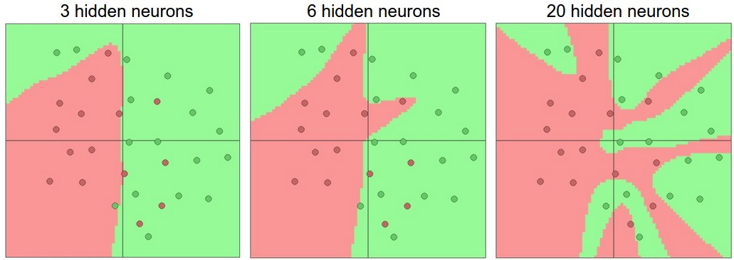
Larger NNs can represent more complicated functions. Circles are data points, colors are classes, decision regions by trained NNs. (ConvNetsJS demo)

• Overfitting: When a high-capacity model learns noise in training data instead of underlying patterns.
  • Left: 1 hidden neuron - too low capacity, underfits.
  • Middle: 3 hidden neurons - good balance.
  • Right: 20 hidden neurons - very high capacity, potentially overfits by creating complex, disjoint decision regions.

When designing a neural network, a core decision is its architecture: how many layers and how many neurons per layer. This directly impacts the network’s “capacity” – its ability to learn and represent complex functions.

The image vividly demonstrates this. A network with too few neurons (1 hidden neuron) has low capacity, and can’t even separate the two classes effectively, leading to underfitting. Conversely, a network with many neurons (20 hidden neurons) has very high capacity. While it can perfectly fit all training data, including noise (like the red points within the green cluster), this can lead to overfitting. The highly complex, jagged decision boundary on the right is a hallmark of overfitting; it may perform poorly on unseen data because it learned the peculiarities of the training set rather than the generalizable patterns. The goal is to find a balance, like the network with 3 hidden neurons, which provides a smoother, more generalizable decision boundary.

Controlling Overfitting: Prioritizing Regularization

Counterintuitive Advice:

• Don’t use smaller networks to prevent overfitting.
• Smaller networks are harder to train effectively with gradient descent; they often converge to “bad” local minima.
• Larger networks have many more local minima, but these tend to be better in terms of actual loss.

Note

Always use as big of a neural network as your computational budget allows!

Preferred Strategy:

• Use a large network to ensure high capacity.
• Control overfitting with robust regularization techniques.

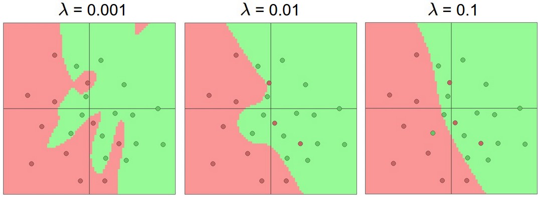
Effects of regularization strength (20 hidden neurons each). Stronger regularization yields smoother decision regions. (ConvNetsJS demo)

This slide presents a crucial, often counterintuitive, piece of advice in neural network design. While small networks seem appealing to prevent overfitting, they are actually harder to train well. Their loss landscapes can be problematic, leading optimizers to get stuck in poor local minima, resulting in suboptimal performance.

Larger networks, despite their higher capacity, offer a more advantageous training landscape. While they have more local minima, these minima tend to yield much better actual loss values. This means a large network, if properly managed, is more likely to converge to a good solution.

Therefore, the recommended strategy is to “go big” with your network architecture (within computational limits) and then actively manage overfitting using regularization techniques. The image on the right illustrates how regularization, like increasing L2 weight decay, can smooth out the decision boundaries even for a large network, making it more generalizable to new data. We will explore various regularization methods like L2 regularization and dropout in detail in later modules.

Summary

• Introduced a coarse model of a biological neuron and its computational counterpart.
• Explored various activation functions (Sigmoid, Tanh, ReLU, Leaky ReLU, Maxout), with ReLU being the most common choice today.
• Defined Neural Networks with Fully-Connected layers, characterized by pairwise connections between adjacent layers.
• Understood how this layered architecture allows for efficient feed-forward computation via matrix multiplications.
• Discussed that Neural Networks are universal function approximators, and why deep layers are still empirically preferred in practice.
• Emphasized using large networks and controlling overfitting with strong regularization rather than limiting network size.

Additional References

• deeplearning.net tutorial with Theano
• ConvNetJS demos for intuitions
• Michael Nielsen’s tutorials