Machine Learning

Image Classification: Data-driven Approach, k-Nearest Neighbor, train/val/test splits

Imron Rosyadi

Introduction to Nearest Neighbor Classifiers

What is Image Classification?

Given: A set of images, each labeled with a single category (e.g., “cat”, “dog”, “car”).

Goal: Train a model to predict the category of new, unseen images.

ECE Relevance:

  • Autonomous Systems: Object detection in self-driving cars.
  • Medical Imaging: Diagnosing diseases from X-rays or MRI scans.
  • Quality Control: Detecting defects in manufacturing.
  • Signal Processing: Classifying radar or sonar signals into object types.

The Nearest Neighbor (NN) Principle

“Birds of a feather flock together.”

The core idea is simple: - Store all training data. - To classify a new point: Find the closest training example. - Assign the new point the label of its closest training example.

Important

How do we define “closest”? We use Distance Metrics!

Defining “Closeness”: Distance Metrics

Common choices for d(I_1, I_2) (distance between images I_1 and I_2):

  1. L1 Distance (Manhattan Distance): \[ d_1(I_1, I_2) = \sum_{p} |I_1(p) - I_2(p)| \]
    • Sums absolute differences across all pixel values.
    • Represents distance if moving only horizontally or vertically.
  2. L2 Distance (Euclidean Distance): \[ d_2(I_1, I_2) = \sqrt{\sum_{p} (I_1(p) - I_2(p))^2} \]
    • Sums squared differences, then takes the square root.
    • Represents the straight-line distance in a multi-dimensional space.

Tip

In ECE, these distances are fundamental for comparing signals or data vectors.

k-Nearest Neighbors (k-NN) Classifier

Beyond a single neighbor

Instead of just one neighbor, k-NN considers the k closest training examples. The label of the new point is determined by a majority vote among its k nearest neighbors.

Key Hyperparameter: k

  • k = 1 is the basic Nearest Neighbor.
  • Choosing k > 1 provides a smoother decision boundary and can reduce sensitivity to noisy data points.

Note

A small k can be sensitive to noise. A large k can blur boundaries.

The Challenge: Choosing Hyperparameters

Hyperparameters are settings that control the learning process, not learned from data.

For k-NN, key hyperparameters include:

  • The value of k.
  • The distance metric (L1, L2, etc.).

Caution

Problem: If we choose k based on how well the model performs on the test data, we are essentially “cheating.” The model would seem to perform better than it would on truly unseen data. This is called overfitting to the test set.

Data Splitting: The Holy Trinity

To correctly tune hyperparameters, we divide our data into three distinct sets:

  1. Training Set (e.g., 60-80%):
    • Used to train the model (e.g., storage for k-NN).
    • The model learns from this data.
  2. Validation Set (e.g., 10-20%):
    • A “fake test set” used to tune hyperparameters.
    • Provides an unbiased estimate of model performance during development.
  3. Test Set (e.g., 10-20%):
    • Used for a single, final evaluation of the chosen model.
    • Provides an unbiased estimate of generalization performance on truly unseen data.

Important

Golden Rule: The Test Set is used only once, at the very end!

Tuning Hyperparameters with a Validation Set

An example with k

# assume we have Xtr_rows, Ytr, Xte_rows, Yte (e.g., 50,000 CIFAR-10 images)
# Xtr_rows is 50,000 x 3072 matrix (image data)
# Ytr are the 50,000 corresponding labels

# 1. Split training data into a smaller training set and a validation set
Xval_rows = Xtr_rows[:1000, :] # Take first 1000 for validation
Yval = Ytr[:1000]
Xtr_rows = Xtr_rows[1000:, :] # Use remaining 49,000 for actual training
Ytr = Ytr[1000:]

# 2. Iterate through different k values and evaluate on the validation set
validation_accuracies = []
for k in [1, 3, 5, 10, 20, 50, 100]: # Try various 'k' values

    # (Imagine a NearestNeighbor class here with a 'train' and 'predict' method)
    # nn = NearestNeighbor()
    # nn.train(Xtr_rows, Ytr) # Model stores the (now smaller) training data

    # Yval_predict = nn.predict(Xval_rows, k = k) # Predict on validation data for current 'k'
    # acc = np.mean(Yval_predict == Yval) # Calculate accuracy

    # --- Simplified for demonstration using placeholder values ---
    # In a real scenario, the above commented lines would compute actual accuracy.
    # For this interactive demo, assume dummy accuracy based on 'k'.
    if k == 1: acc = 0.38
    elif k == 3: acc = 0.42
    elif k == 5: acc = 0.44
    elif k == 10: acc = 0.41
    elif k == 20: acc = 0.35
    elif k == 50: acc = 0.28
    elif k == 100: acc = 0.20
    # --- End simplified part ---

    print(f'k = {k}: accuracy = {acc:.4f}')
    validation_accuracies.append((k, acc))

# 3. Choose the 'k' that gave the best accuracy on the validation set
best_k = max(validation_accuracies, key=lambda item: item[1])[0]
print(f"\nBest k on validation set: {best_k}")

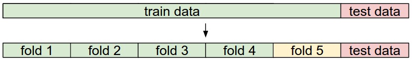
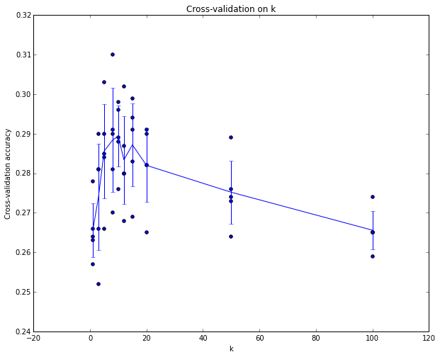
When Validation Data is Small: Cross-Validation

  • Problem: If your dataset is small, a single validation split might not be representative (noisy estimate).
  • Solution: Cross-validation provides a more robust estimate of performance for hyperparameter tuning.

How it works (e.g., 5-fold CV):

  1. Divide the training data into N equal “folds” (e.g., 5).
  2. Iterate N times:
    • Use N-1 folds for training.
    • Use the remaining 1 fold for validation.
    • Record performance for the current hyperparameter setting.
  3. Average the performance across all N iterations.

Tip

Common folds: 3, 5, or 10. More folds offer a better estimate but are more computationally expensive.

Practical Considerations for Data Splits

  • Typical Split Ratios:
    • Training: 50-90%
    • Validation: 10-20%
    • Test: 10-20%
  • When to favor Cross-Validation over a single split:
    • Small dataset size (validation set would be too small).
    • If a very accurate estimate of hyperparameter performance is crucial.

Note

Cross-validation is computationally more expensive. Choose between a single validation split and cross-validation based on dataset size, available computational resources, and the number of hyperparameters to tune.

Pros of Nearest Neighbor Classifiers in ECE

  1. Simplicity & Interpretability:

    • Easy to understand and implement.
    • Can provide insight into why a decision was made (by looking at neighbors).
    • Useful for quick prototyping in ECE.
  2. No Training Time:

    • The model merely stores the training data.
    • “Lazy learning” – computation happens during inference.
    • Can be beneficial for systems where initial training needs to be minimal or dynamic.
  3. Non-parametric:

    • Makes no assumptions about the underlying data distribution.
    • Can model complex decision boundaries.

Cons of Nearest Neighbor Classifiers in ECE

  1. High Test-Time Cost:
    • Classifying a new point requires comparing it to all training points.
    • Critical for ECE: Unsuitable for real-time applications or embedded systems with large datasets.
  2. Storage Requirements:
    • Must store the entire training dataset.
    • Problematic for memory-constrained devices (e.g., IoT, edge AI).
  3. Curse of Dimensionality:
    • Distances become less meaningful in high-dimensional spaces.
    • This is a major issue for image data, as we’ll see next.

The Curse of Dimensionality & Image Data

Why pixel-based distances fail for images

Pixel-based L1 or L2 distances often correlate more with background and general color distribution than with semantic content.
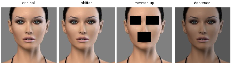
Warning

The image on the left is the original. The three images next to it are all equally far away by L2 pixel distance. Notice: The L2 distance suggests they are equally similar, despite huge perceptual differences.

  • A truck and a horse can be “closer” if they share a similar background or lighting.
  • Semantic meaning (“what the image is”) is lost in raw pixel comparisons.

Visualizing Failure: t-SNE Embedding of CIFAR-10

t-SNE (t-Distributed Stochastic Neighbor Embedding) helps visualize high-dimensional data in 2D or 3D, preserving local neighborhood structures.

Important

Observation: Images nearby in this embedding (meaning they are pixel-wise similar) are clustered by background/color, not by their semantic class (e.g., “dog”, “cat”, “car”).

Towards Smarter Features: Introduction to Convolution

Why ECE needs better feature extraction for images

The failure of pixel-wise distances indicates a need for more robust feature representations. ECE Connection: Image processing often involves filtering — a form of feature extraction.

Note

Convolution is a fundamental operation for extracting meaningful features from image and signal data.

How it works:

  • A kernel (small matrix/filter) slides over the input image.
  • At each position, it computes element-wise products and sums them.
  • This generates a new “feature map” highlighting specific patterns (edges, textures).

Summary

  • Image Classification: Assigning labels to images.
  • Nearest Neighbor (k-NN): Simple, non-parametric classifier that uses proximity in feature space. Key hyperparameters: k and distance metric.
  • Hyperparameter Tuning: Critical for generalizing to new data. Avoid test set overfitting.
  • Data Splits: Use Training, Validation, and Test sets. Test set is for final evaluation only.
  • Cross-Validation: Robust tuning for smaller datasets.
  • k-NN Limitations for Images: High test-time cost, storage, and curse of dimensionality (pixel-wise distances are inadequate).
  • Future Direction: Need for better feature extraction (e.g., Convolution).

Applying k-NN in Practice (ECE Guidelines)

If you consider k-NN (perhaps not for images, but for other sensor data):

  1. Preprocess Data: Normalize features (e.g., zero mean, unit variance). Critical for distance-based methods.
  2. Dimensionality Reduction: For very high-dimensional ECE data (e.g., spectral analysis, multi-sensor arrays), consider PCA, NCA, or Random Projections.
  3. Data Splitting: Robustly split data into train/validation/test. Use cross-validation if data is sparse or hyperparameters are complex.
  4. Hyperparameter Search: Systematically evaluate k and distance metrics on the validation set.
  5. Accelerate Retrieval: For speed-critical ECE applications, explore Approximate Nearest Neighbor (ANN) libraries like FLANN.
  6. Final Evaluation: After selecting the best hyperparameters, evaluate the model once on the untouched test set. Report this performance.

Further Reading