Machine Learning

5. Deep Learning: AE, TL

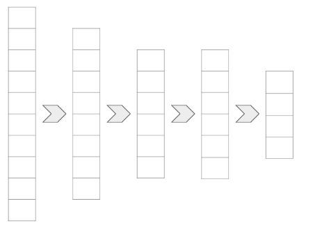
Imron Rosyadi

Autoencoders

What Is an Autoencoder?

A neural network designed to learn an efficient data encoding (compression)
and then reconstruct the input data from that encoding (decompression).

Tip

Core Idea: Learn a compressed, “latent” representation of data without supervision.

First things first, what is an autoencoder? It is a model that learns how to encode data and then decode data.

Let’s look at a visualization.

Encoder

The encoder is a neural network that transforms input data into a smaller,
lower-dimensional representation.

• Goal: Reduce data dimensionality while retaining essential information.
  
• Layers: Can use dense, convolutional, pooling layers, etc.
  
• Output: A compressed “latent space” representation.
  

Encoding looks a whole lot like the neural networks that we have already seen, and that’s because it is. The encoder is a neural network that starts out with some input data and outputs a smaller form of that data. The encoder can use dense layers, convolutional layers, pooling layers, and more.

The goal of the encoder is to take some form of input data and reduce it down to a smaller representation.

But there has to be some way to know if this smaller representation is useful. We do that with the decoder.

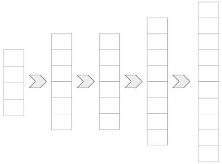
Decoder

The decoder performs the reverse operation of the encoder.

• Input: The compressed latent representation from the encoder.
  
• Goal: Reconstruct an approximation of the original input data.
  
• Method: Expands the data back to its original dimensions.
  

As you might expect, the decoder does the opposite of the encoder. The decoder starts with a compressed representation of the data and inflates it back to the original size.

We haven’t really seen this before. The networks we have built tend to get narrower as data flows through them. This widening is less common. Sure, we could add wider and wider dense layers in a deep neural network, but it isn’t common to see outside of this context.

How do we do this?

Decoder: Upsampling

To expand the data in the decoder, we use upsampling techniques.

• Concept: Reverse of pooling; expands input dimensions.
  
• UpSampling2D: Commonly used in TensorFlow Keras for image data.
  
• Example: Doubles spatial dimensions (e.g., 4x4 to 8x8).
  

tf.keras.layers.UpSampling2D(
    size=(2, 2)
)

conv2d_3 (Conv2D)            (None, 4, 4, 16)          2320      
_________________________________________________________________
up_sampling2d (UpSampling2D) (None, 8, 8, 16)          0      

We use upsampling to add wider dense layers and create the decoder. You can think of upsampling as the reverse of the pooling layers we used in the convolutional neural networks we created for classification. While a pooling layer shrinks its input, the upsampling layer expands its input.

In TensorFlow Keras we’ll use the UpSampling2D layer to decode our encoded data.

In the example on this slide, you can see a convolutional layer that outputs a 4x4x16 matrix. The upsampling layer doubles the first two dimensions to 8x8x16.

Autoencoder

Combining the encoder and decoder forms an autoencoder.

• Encoder: Learns efficient data representation.
  
• Decoder: Reconstructs data from the encoded representation.
  
• “Lossy” Compression: Output is an approximation, not exact replica.

Important

The autoencoder aims to reconstruct its own input.

What do you get when you mix an encoder and a decoder? An autoencoder!

The encoder finds an efficient representation for the data. The decoder is able to revive some approximation of the original data from the encoded data.

This is “lossy” compression. The output of the model is not typically exactly what was put in, but is hopefully a reasonable approximation.

What Are Autoencoders Good For?

• Lossy Data Compression: Efficiently reduce data size.
  
• Non-linear Principal Component Analysis (PCA): Discover underlying data structure.
  
• Data Denoising/Cleaning: Remove noise or artifacts from data.
  
• Feature Learning: Extract meaningful features for other ML tasks.
  
• Anomaly Detection: Identify data points that deviate from learned patterns.

Obviously autoencoders are good at lossy data compression. Once trained, the encoder part of the model can be used to compress our input data. The decoder can then later be used to expand that data to a version that is close to the original.

Another application is principal component analysis. If you think about what an autoencoder is doing, it is reducing input data down into the minimal amount of information required to then revive that data. It is finding principal components using a neural network. You can train the model and then use the encoder to reduce the dimensionality of your data before feeding it into another model.

Another interesting application is data cleaning. Autoencoders can be used to remove noise from data. In our lab we’ll remove static and watermarks from images. Admittedly, there is some data loss, but it is still an interesting application.

Keras Model: Building the Encoder

Utilize the Keras Model class for flexible architecture.

from tensorflow.keras.layers import Conv2D, MaxPool2D, UpSampling2D, Input
from tensorflow.keras.models import Model

# Define input layer
input_layer = Input(shape=(28, 28, 1), name='input_image')

# Encoder path
conv_layer = Conv2D(32, (3, 3), activation='relu', padding='same')(input_layer)
latent_layer = MaxPool2D((2, 2), padding='same')(conv_layer)

# Define the encoder model
encoder = Model(input_layer, latent_layer, name='encoder')

print(encoder.summary())

Note

The latent_layer represents the compressed output of the encoder.

You could build an autoencoder with a standard Sequential model, but often you’ll want to use the encoder and decoder separately. In order to do this, we can use the Keras Model class.

In this example we build an input layer and pass it to a convolutional layer, which is then passed to a pooling layer. The input and output layers are then passed to the Model.

You might also notice that we called the output of the encoder the “latent layer.” This is a common term used to identify the intermediate data representation that is output by the encoder and input to the decoder.

Keras Model: Assembling the Autoencoder

Connect encoder and decoder using the Keras Functional API.

from tensorflow.keras.layers import Conv2D, MaxPool2D, UpSampling2D, Input
from tensorflow.keras.models import Model

# Example placeholder for decoder output (in a real model, this would be built from latent_layer)
# For this example, let's just make a simple decoder structure
latent_input = Input(shape=(14, 14, 32), name='latent_input')
conv_decoder = Conv2D(32, (3, 3), activation='relu', padding='same')(latent_input)
up_sample = UpSampling2D((2, 2))(conv_decoder)
output_layer = Conv2D(1, (3, 3), activation='sigmoid', padding='same')(up_sample) # Assuming 1-channel output like original input

# Define the encoder model (as on previous slide)
input_autoencoder = Input(shape=(28, 28, 1), name='input_image_autoencoder')
encoder_conv = Conv2D(32, (3, 3), activation='relu', padding='same')(input_autoencoder)
latent_encoded = MaxPool2D((2, 2), padding='same')(encoder_conv)
encoder = Model(input_autoencoder, latent_encoded, name='encoder')

# Define the decoder model
decoder = Model(latent_input, output_layer, name='decoder')

# Connect them to form the autoencoder
autoencoder = Model(
    input_autoencoder,
    decoder(encoder(input_autoencoder)),
    name="autoencoder"
)

print(autoencoder.summary())

Tip

Training the autoencoder model simultaneously trains both the encoder and decoder sub-models.

To build an autoencoder, you create an encoder and a decoder. The encoder accepts an input layer and outputs a latent layer. The decoder accepts a latent layer and outputs an output layer.

The encoder and decoder are stitched together into a third model, the autoencoder. Notice that the autoencoder accepts the input layer and passes it directly to the encoder. The encoder is the input to the decoder (via the latent layer).

When the autoencoder is trained, the encoder and decoder are also trained and can be used separately.

Interactive Convolution Visualization

Explore how a 2D convolution filter processes an input matrix.
Adjust filter size and visualize the output.

viewof input_val = Inputs.range([0, 10], {step: 1, value: 5, label: "Input Matrix Base Value"});
viewof filter_size = Inputs.select(["3x3", "5x5"], {value: "3x3", label: "Filter Size"});

Note

This visualization shows a single convolution operation with a simple filter.

Here we visualize a simplified 2D convolution. You can adjust the base value of the input matrix and the size of the filter. The input matrix is a simple gradient. The filter matrix is a basic edge detection or blur kernel. The output feature map shows the result of applying the filter across the input.
Convolution involves sliding the filter over the input, performing element-wise multiplication, and summing the results for each position. This process helps detect features like edges or textures in the input data.

Your Turn!

Now it is your turn to apply what you’ve learned about autoencoders.
In the lab, you will work through examples of:

• Using an autoencoder for image compression.
  
• Applying autoencoders for denoising (e.g., removing static from images).
  
• An exercise to remove a watermark from a video or image.

What specific ECE applications do you envision for autoencoders, beyond those discussed?

Now it is your turn. In this lab we will walk through examples of using an autoencoder for compression and for removing static. Our exercise will be to remove a watermark from a video.

Image Classification Project

Identifying Pneumonia from X-rays

This project consolidates your knowledge of image classification.
You will apply various techniques learned throughout the course.

Note

Focus on building, evaluating, and tuning models for a real-world medical imaging task.

We are nearing the end of the classification track. We’ve learned quite a bit. In the last few labs we’ve created binary and multiclass classifiers. We’ve used scikit-learn and TensorFlow to create various models we then evaluated and tuned.

In this final project, you’ll get to show off what you’ve learned in one large project.

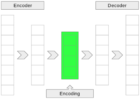
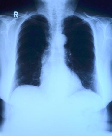
Image Classification Project: Chest X-rays

You will work with a dataset of chest X-ray images.

• Task: Classify images as either NORMAL or PNEUMONIA.
  
• Source: Dataset from Kaggle, pre-divided for training, testing, and validation.
  
• Relevance: Demonstrates ML application in medical diagnostics.
  

In the lab we’ll download a dataset from Kaggle. The dataset contains images of x-rays of patient lungs. Some of the images are classified as having pneumonia, while others are classified as normal.

Review: What is Convolution?

• Definition: A mathematical operation involving two functions to produce a third.
  
• Image Processing: A “filter” (kernel) slides over an input image.
  
• Process: Element-wise multiplication of filter with image region, then sum.
  
• Goal: Detect specific features (e.g., edges, textures) in the image.
  
• Parameters: Filter size, stride, padding.
  

flowchart LR
    subgraph "Input Image"
        A["Pixel Grid"]
    end

    subgraph "Filter (Kernel)"
        B["Small Matrix"]
    end

    subgraph "Operation"
        C(("Slide & Multiply-Add"))
    end

    subgraph "Output"
        D["Feature Map"]
    end

    A -- "Apply Filter" --> C
    B -- "Over Region" --> C
    C --> D

    style A fill:#cef,stroke:#333,stroke-width:2px
    style B fill:#fec,stroke:#333,stroke-width:2px
    style C fill:#ccf,stroke:#333,stroke-width:2px
    style D fill:#cfc,stroke:#333,stroke-width:2px

@Exercise(5 minutes) {
Have students discuss convolution. It is a process of passing a filter (kernel) over an image and computing new pixel values. This process involves multiplying the values in the image by those in the filter and adding them up. You need to know the size of your filter and the stride. The goal is to detect features in the image. Remind students that we saw simple kernels that were line detectors.
}

Review: Convolutional Neural Network (CNN) Architecture

• Key Components:
  • Convolutional Layers: Feature extraction using filters.
    
  • Pooling Layers: Downsampling to reduce dimensionality and computational cost.
    
  • Activation Functions: Introduce non-linearity (e.g., ReLU).
    
  • Fully Connected Layers: Classification based on extracted features.
    
• Tunable “Knobs”:
  • Number of layers, layer order.
    
  • Filter size, number of filters, stride.
    
  • Pooling size, type of pooling.
    
  • Activation functions (e.g., ReLU, Sigmoid for output).
    
  • Dropout rates, learning rate, batch size.

Exercise(5 minutes) {
Have students discuss CNNs. In general, there are convolutional layers and pooling layers. Then the information is fed into a typical fully-connected neural network. Furthermore, an important choice the user needs to make is which activation function to use. Since this is a binary classification task, it is useful to use the sigmoid function on the final output layer. Relu works well on the other layers.
}

Image Classification Project: Dataset Structure

The dataset is pre-organized into standard machine learning splits.

chest_xray/
     ├── test/
     │       ├── NORMAL/
     │       └── PNEUMONIA/
     ├── train/
     │       ├── NORMAL/
     │       └── PNEUMONIA/
     └── val/
             ├── NORMAL/
             └── PNEUMONIA/

• train set: Used for model training.
  
• test set: For hyperparameter tuning and model selection.
  
• val set: Final, unbiased evaluation of model generalization.

The images in the dataset are already divided into test, train, and validation sets. The training set is, of course, used for training your model. The testing dataset should be used to adjust model hyperparameters, shape, etc. Once you have found a model that tests well, check it against the validation dataset. That will serve as one final test for the ability for your model to generalize.

Image Classification Project: Tips for Success

• Enable GPU: Significantly speeds up training for image models.
  • In Google Colab: Runtime > Change runtime type > Hardware accelerator > GPU.
    
• Perform Exploratory Data Analysis (EDA):
  • Verify dataset integrity and structure.
    
  • Check for image dimensions, class balance, and potential anomalies.
    
• Data Augmentation: Consider techniques like rotation, flipping, zooming to expand training data.
  
• Transfer Learning: Explore pre-trained models for faster convergence and better performance.

What challenges do you anticipate when working with medical image data?

First tip: enable GPU in Google Colab. This dataset tends to train significantly faster if you enable GPU in the runtime.

Also, perform EDA on your dataset. The dataset may have duplication, undocumented folders, etc.

Your Turn!

Now, apply your skills to the Image Classification Project.
Good luck building a robust pneumonia detection model!

What strategies will you prioritize for model evaluation and fine-tuning?

And with that, it is your turn to work on the lab.

Transfer Learning

Leveraging Pre-trained Models

Concept: Reusing a pre-trained model as a starting point for a new task.

• Traditional ML: Models trained from scratch on specific datasets.
  
• Transfer Learning: Utilizes knowledge gained from a large, general dataset.
  
• Benefit: Accelerates training, improves performance with limited data.
  

Important

Why train from scratch when you can stand on the shoulders of giants?

Most of the models we have trained so far have been trained from scratch. We start with a randomly-weighted model and then use large amounts of data and many, many epochs over that data in order to build a reasonable model.

But is that how we learn?

Transferring Knowledge: Human Analogy

Just as humans learn by building upon existing knowledge,
ML models can benefit from “transferred” insights.

• Direct Learning: Observing examples directly.
  
• Knowledge Transfer: Gaining insights from others’ experiences or related domains.
  
• Efficiency: Speeds up the learning process for new, related tasks.
  

Well, yes and no.

We do indeed learn in self-guided ways by looking at examples. But we also learn through the transfer of knowledge. Others can provide insights that can be used to accelerate our learning process.

Transferring Knowledge: The Zebra Example

Imagine identifying a zebra:

• Knowns: Horse shape, tiger stripes, penguin colors.
  
• Transferred Knowledge: Combining these known features accelerates zebra identification.
  
• ML Parallel: A model good at general image recognition can quickly adapt to new categories.
  

Let’s say we already know what a horse, tiger, and penguin are. If we wanted to learn how to identify a zebra, we could look at pictures of zebras. Or, someone might tell us that a zebra is the shape of a horse, has the coat patterns of a tiger, and the colors of a penguin. This would greatly accelerate our ability to identify zebras, even if we only had a handful of pictures of zebras to study.

Transfer learning is a similar idea. A model that can already identify some classes of data can be extended to fit a different problem that we are trying to solve. The base model is already good at finding key features. The new model can utilize this ability and perform better and faster than if it was trained from scratch.

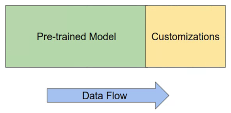
Transfer Learning: High-Level Overview

Typically involves attaching new layers to a pre-trained base model.

• Pre-trained Model: Base model with learned weights (e.g., ImageNet classifier).
  
• Customization Model: New, untrained layers added on top.
  
• Data Flow: Input goes through pre-trained model, then into new layers.
  
• Output: The final prediction from the new layers.
  

At a very high level, transfer learning can look a lot like adding an extra few layers to the end of a pre-trained model.

In this diagram the pre-trained model is an existing model that has been trained and performs acceptably well. This model has persisted weights that are packaged and loaded with the model.

The customizations model is a new set of untrained layers. They have random, or at least naive, initial weights. These weights still need to be learned through training.

As you can decipher from the data flow arrow, data typically still enters the model through the pre-trained input layer. However, the output layer of the pre-trained model then feeds the new model. The final output is the output layer of the new model.

Do You Retrain the Pre-Trained Model?

The decision to retrain (fine-tune) the pre-trained model’s weights depends on several factors:

• “Freezing” Weights:
  • Usually “No”: If new data is small or classes don’t largely overlap.
    
  • Benefit: Prevents overfitting, faster training of new layers.
    
• Fine-tuning Weights:
  • Sometimes “Yes”: If new data is large and similar to original training data.
    
  • Method: Unfreeze some or all layers and train with a very small learning rate.
    
• Layer-Specific Freezing: Often, layers closer to the input are frozen, while later layers are fine-tuned.

This begs the question: Do you re-train the pre-trained model?

The answer is usually “no” but not always.

If the data you have to train your new model is similar in size or larger than the data used to train the pre-trained model, and if the classes that they identify largely overlap, then it may be worthwhile. Otherwise it is advisable to “freeze” the pre-trained model and not update the weights.

This freezing can be for the whole model or for only a few specific layers. Typically those layers closer to the input layer are frozen.

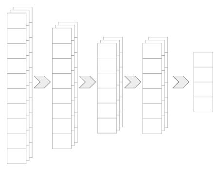
Which Output Layer to Use?

When using a pre-trained model, we typically don’t use its final classification layer.

• Problem: Final layers usually flatten data into class-specific vectors.
  
• Solution: Use an intermediate high-dimensional layer as the output from the pre-trained model.
  
• Benefit: Provides rich feature representations for the new custom layers.
  

We also need to think about which layer is actually the output layer from a pre-trained model.

In most classification problems, we have multiple layers of high-dimensional matrices. But then at the very end of the model, we flatten the data down to a vector of class-estimates.

We don’t want to flatten the data before feeding it to our extended model, so instead we need to use an intermediate high-dimensional layer.

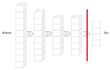
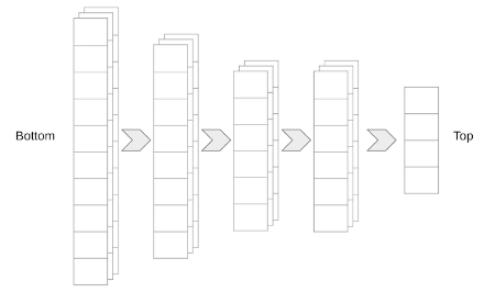
Model Terminology: “Bottom” and “Top”

Understanding these terms helps when configuring pre-trained models.

• “Bottom”: Refers to the input layers of the model.
  
• “Top”: Refers to the output layers of the model.

This convention often comes from how models are diagrammed, with input at the bottom and output at the top.

We need to introduce a little modelling terminology at this point. You sometimes hear about the “bottom” or “top” of a model. Which end is which?

Many papers illustrate models with the input layer at the bottom and the output layer at the top of diagrams. For this reason, culture now dictates that the “bottom” of a model is the input, and the “top” of a model is the output.

include_top: A Key Parameter

Many pre-trained models (e.g., in Keras) offer an include_top parameter.

• include_top=True (default): Includes the original classification layers.
  
• include_top=False: Excludes the original classification layers.
  • Benefit: Provides a high-dimensional feature extractor.
    
  • Use Case: Ideal for building custom classifiers on top.
    

This terminology is important because some models allow you to choose to include the “top” of the model or not. If you leave out the top, then you get a higher-dimensional input for your custom model, which is typically a good thing.

Your Turn!

Now, let’s put transfer learning into practice.

You will use MobileNetV2, a powerful pre-trained model,
to build a network capable of classifying cats and dogs.

What advantages do you expect from using MobileNetV2 compared to training from scratch for this task?

Now we’ll attempt a little transfer learning of our own. We’ll use MobileNetV2, which can classify 1,000 classes, to build a network that can reliably classify cats and dogs.