Machine Learning

5. Deep Learning: CNN, RNN, NLP

Imron Rosyadi

Convolutional Neural Network

The Biological Inspiration: Visual Cortex

In the 1960s, research by David Hubel and Torsten Wiesel revealed how the visual cortex processes visual information.

• Neurons respond to specific regions of the visual field.
  
• Each neuron has a “receptive field.”
  
• Spatially close neurons have similar, overlapping receptive fields.
  

Like neural networks, convolutional neural networks were inspired by biology.

In the 1960s, David Hubel and Torsten Wiesel showed that the visual cortex in cats and monkeys contain neurons that fire individually in response to small regions in the field of view.

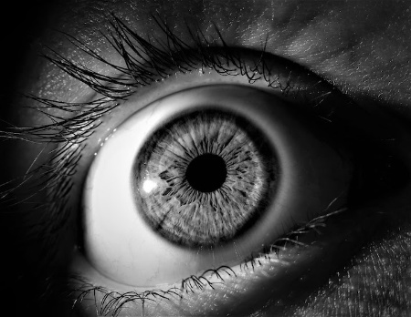
Receptive Fields and Image Formation

Our visual system integrates information from these small receptive fields.

This process forms the complete images we perceive.

This biological mechanism provided a key inspiration for Convolutional Neural Networks (CNNs).

For a given neuron, the visual space that affects whether or not that neuron will fire is known as its “receptive field.”

Neurons that are spatially close together often have similar and overlapping receptive fields.

Our eyes and brains then take the information from each of these small receptive fields and meld them together into the images that we see.

Introduction to Convolutional Neural Networks (CNNs)

Inspired by the visual cortex, CNNs emerged in the 1980s.

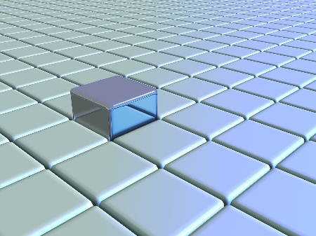
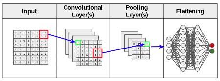
CNNs are specialized neural networks for processing structured grid data, like images.

They incorporate unique layer types:

• Convolutional Layers
  
• Downsampling Layers
  
• Pooling Layers
  

In the 1980s researchers were inspired by the visual cortex and used these ideas to create convolutional neural networks.

A convolutional neural network is simply a neural network with additional (or different) types of layers. There are convolutional layers, downsampling layers, and pooling layers.

CNN Architecture Flexibility

The power of CNNs lies in their flexible architecture.

Different combinations and ordering of layers lead to varied results.

This allows for optimization based on the specific task.

You can stack different numbers of these layers in various orders to achieve different results during training.

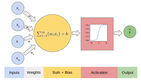
Recall: The Perceptron

The simplest building block of a typical neural network.

A basic computational unit that processes inputs to produce an output.

Recall the simplest building block for a typical neural network: the perceptron.

Issues with Multi-Layer Perceptrons (Plain ANNs) for Images

Sensitivity to Input Changes:

• Small shifts in image data can drastically alter learned parameters.
  
• E.g., a cat’s position in an image should not change its recognition.
  

If we are dealing with image data, small and often insignificant changes to the training data can yield large and often incorrect changes to the learned parameters in the model.

For example, consider a problem where you want to identify a cat in an image. If the cat is translated to a different part of the image, then the model will adjust different weights to recognize the cat. But the cat being on the left or right of an image isn’t really a defining feature of a cat, right? We’d prefer to recognize things like ears, fur, etc.

CNNs help us solve this problem.

CNNs: A Solution for Image Data

CNNs introduce specialized layers to address the limitations of plain ANNs for image processing.

The processed output then feeds into a fully connected neural network.

In a convolutional neural network, we first feed our data into convolutional, downsampling, and pooling layers. The results are then fed into a fully connected neural network like we have seen before.

Convolution: Analyzing Pixel Influence

A fundamental operation in CNNs.

It uses a filter (also called a kernel, mask, or convolution matrix) to analyze the influence of nearby pixels.

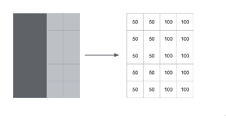
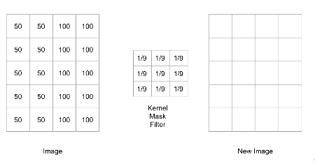
Convolution Example: Input Image

Consider a simple image: a rectangle with two shaded halves.

Pixel intensities are represented numerically.

Let’s look at a simple example. Imagine we have the image on the left. It’s just a rectangle with two halves shaded different colors.

The intensity of each pixel is recorded on the right. This is how we typically work with image data.

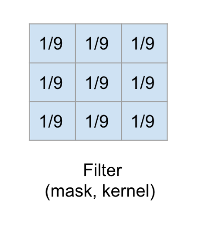
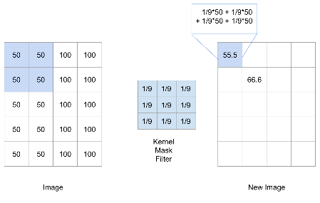
Convolution Example: Blurring Filter

We apply a 3x3 filter designed to create a blurring effect.

Each element in the filter has a specific weight.

We’ll apply this 3x3 filter to the image.

It’s a filter that adds a blurring effect.

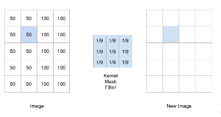
Convolution Example: Filter Application

The filter is applied by sliding it over the image.

At each position, it computes a new pixel value.

We’ll apply this 3x3 filter to the image.

It’s a filter that adds a blurring effect.

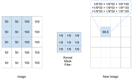
Convolution Example: Calculating a New Pixel Value

To calculate the new value for a pixel:

1. Center the filter on the target pixel.
   
2. Multiply corresponding values from the filter and the image.
   
3. Sum the products.
   

Let’s use the 3x3 filter to calculate the new value for this pixel.

Convolution Example: Result of Blurring

The new pixel value is an average of its neighbors.

This averaging effect reduces sharp intensity changes, leading to blurring.

First we think of centering the filter on the pixel. Then we multiply the values in the filter by the values in the image. And finally, we add up the result.

As you can see, the new pixel value is slightly lower than 100, but it’s higher than 50. So the intensity is getting muted a little. This is because our filter is averaging the intensity of all the pixels around the center point. That is why this filter results in a blurring effect.

Handling Edges: Padding

When the filter reaches the image edge, padding is often used.

Commonly, the original image is padded with zeros around its borders.

You may be wondering what happens if we’re at the edge. There are different ways to handle this. But it’s common to pad the original image with 0’s around the edges. That way, those values drop out in the average.

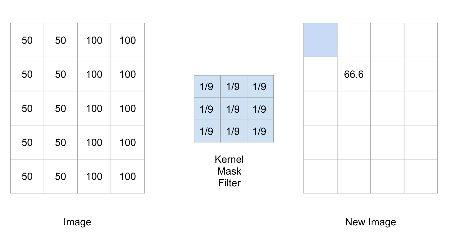
Edge Handling: Relevant Filter Area

The padding ensures the filter can be centered on edge pixels.

Only the part of the filter overlapping the original image contributes to the sum.

Here you can see that we only used the part of the filter that is relevant to the image.

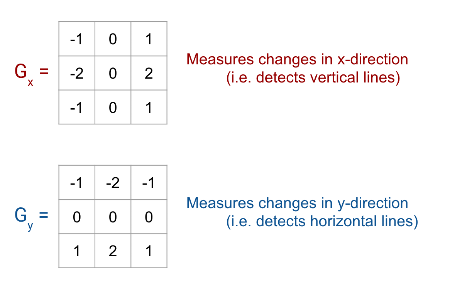
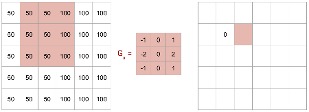
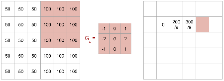
Line Detectors: Gx and Gy Kernels

These kernels are designed to detect sharp intensity changes, indicating lines or edges.

• \(G_x\): Detects vertical lines.
  
• \(G_y\): Detects horizontal lines.
  

Here are two very common kernels that can be used to detect lines in an image.

Overall the goal is to detect sharp changes in intensity. Let’s see how this works by doing an example with G\(_{x}\).

Line Detector Example: Input Image

An image with a vertical line where shading changes.

We will apply the \(G_x\) kernel to detect this line.

On the left we have an image that is similar to the previous example. There is a line down the center, where the shading changes color. Let’s see if the kernel G\(_{x}\) can detect this line.

Calculate the pixel on the right.

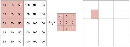
Line Detector Example: First Pixel

Applying \(G_x\) to the first 3x3 block yields 0.

No intensity change within this block.

We get 0. There are no changes in intensity in the 3x3 block that is highlighted in the original image.

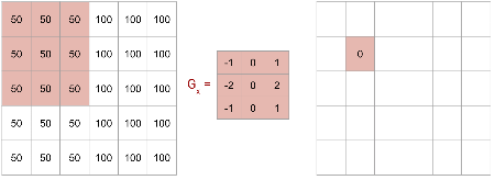
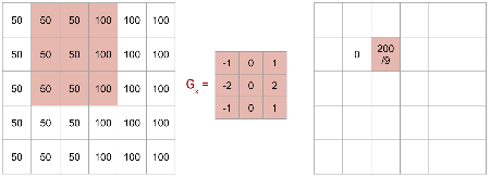
Line Detector Example: Shifting Right

Shifting the \(G_x\) kernel one pixel to the right.

The kernel now straddles the intensity change.

Now let’s move one pixel to the right.

Line Detector Example: Detecting the Edge

The calculation results in a non-zero value (\(200/9\)).

This indicates the presence of a vertical edge.

We get 200/9.

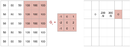
Line Detector Example: Further Shift

Shifting the \(G_x\) kernel one more pixel to the right.

The kernel is now fully on the right side of the edge.

Again move one pixel to the right.

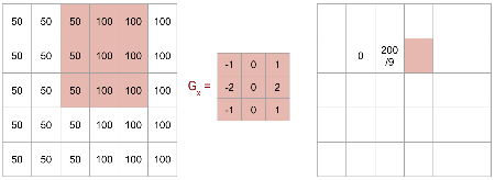
Line Detector Example: Another Non-Zero

The calculation results in \(300/9\).

This continues to highlight the edge region.

We get 300/9.

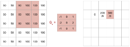
Line Detector Example: Past the Edge

Shifting the \(G_x\) kernel one final pixel to the right.

The kernel is now past the intensity change.

Finally, let’s move one more pixel to the right.

Line Detector Example: Back to Zero

The calculation returns 0 again.

This demonstrates that \(G_x\) effectively detects vertical lines by identifying sharp horizontal intensity transitions.

And again we get 0.

Thus, we see that a vertical line was detected when the intensity changed in the original image.

CNNs Learn Features

In CNNs, the kernel values are learned during training.

The network automatically identifies important features.

We don’t explicitly tell the model what to look for (e.g., “vertical lines”).

This type of convolution happens in the convolutional layers of a neural network. The values in the kernels are parameters that will be learned during training. Thus, the specific features in the images that the kernels are testing for is something that the model “learns.” In other words, you don’t say “Hey model, test for vertical lines.” Instead, the model identifies the features that are important to test for.

Pooling

A downsampling technique often applied after convolution.

Objective: Reduce data size without losing critical information.

1. Window Size: Select a region (e.g., 2x2 or 3x3).
   
2. Stride: Define movement step (e.g., 2 pixels).
   
3. Window Movement: Slide the window across filtered images.
   
4. Value Selection: Take the maximum (Max Pooling) or average (Average Pooling) value within each window.

Pooling is a type of downsampling that often occurs after convolution. The goal is, without losing much information, to reduce the size of the training data before it goes into the fully connected network.

Hyperparameters in CNNs

While CNNs learn many parameters, users define several key hyperparameters:

Convolution:
- Number of filters (features)
- Size of filters

Pooling:
- Window size
- Stride

Fully Connected Layers:
- Number of nodes

Also, the number and order of each layer type.

While a convolutional neural network learns MANY parameters, there are also several hyperparameters that are chosen by the user. Here are the main ones. But as with our previous neural networks, the user can also choose the optimizer, activation function, etc.

Your Turn: CNNs in Practice

In the lab, you will build and experiment with a Convolutional Neural Network.

You’ll apply these concepts to a practical image classification task.

Now it’s your turn to build a CNN in the lab.

Recurrent Neural Networks (RNNs)

Beyond Feedforward: Introducing RNNs

Previous deep neural networks were primarily feedforward.

• Data flows in one direction.
  
• Weights adjusted via backpropagation.

Recurrent Neural Networks (RNNs) introduce a new dynamic.

• Not strictly feedforward.
  
• Designed for sequential data.
  

Note

RNNs excel in tasks where the order of data points is crucial, such as time series or natural language.

We have encountered numerous deep neural networks throughout this course. In previous tracks we’ve covered, training data flowed through the network (feedforward), and then adjustments were made to the weights in the network from the last layer through the first (backpropagation).

Just to name a few, we’ve used dense layers, dropout layers, convolutional layers, and pooling layers. In this unit we will learn about recurrent neural networks, which are not strictly feedforward networks.

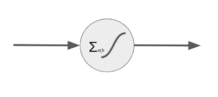
The Feedforward Neuron

• Receives inputs from the previous layer.
  
• Multiplies inputs by weights, adds bias.
  
• Passes sum through an activation function.
  
• Output goes to the next layer.
  

Here we see a typical feedforward neuron. Depending on the size of the layers before and after, one or more weights feed into the neuron. These are multiplied by the bias, summed, and then passed through an activation function. The resultant value is then passed to the nodes in the next layer of the network.

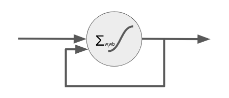
The Recurrent Neuron

A feedforward neuron with a crucial addition:

• Its output feeds back into its own inputs.
  
• This creates a “memory” over time.
  
• Allows processing of sequential data.
  

Here is a recurrent neuron. You can see that the recurrent neuron looks a lot like a feedforward neuron, except that it also feeds its output back into its inputs.

Imagine we have a fully connected layer that is 10 nodes wide before this neuron. In a typical feedforward, fully-connected network, we would expect 10 inputs, one for each of the nodes in the previous layer. In this case we’ll actually have 11 inputs: one for each of the nodes in the previous layer and the output of the node itself.

What does this do? This gives the neuron memory over time. It allows you to pass a series of data points into the network over time.

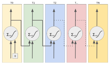
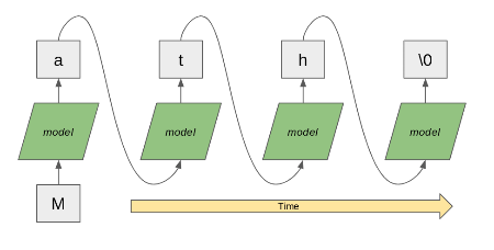
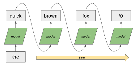
Unrolling a Recurrent Neuron Over Time

Visualizing the data flow:

• Starts with a seeded input (often zero).
  
• At each time step, it processes current input and its own previous output.
  
• Passes data to the next layer and forward in time to itself.
  

This is what it would look like to “unroll” the flow of data through a recurrent neuron over time. You can see that it typically starts out with a seeded input value of zero for its backfeed. At each point in the series, the neuron both passes data to the next layer of neurons and passes data forward in time to itself the next time it fires.

Also note that we’re looking at a single neuron in a layer with one input and one output. In reality you’ll have wide layers, so imagine multiple recurrent nodes side by side, each with multiple inputs and outputs.

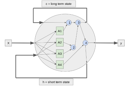
The Long Short-Term Memory (LSTM) Neuron

Addresses the “short memory” problem of standard RNNs.

• Passes two weights back to itself:
  • Long-term memory
    
  • Short-term memory
    
• Uses “gates” (forget, input, output) to control information flow.
  

With a typical recurrent neural network, the network tends to have a very short memory. As the sequences passing through the network get longer, the network forgets what it first saw. There have been a few strategies to get around this, one of which is the “long short term memory” (LSTM) neuron.

On this slide you can see a very simplified LSTM cell. If you look at the horizontal center, you can see the standard neuron: X-in, y-out. However, instead of having a single feedback like a standard recurrent neuron, this neuron passes two weights back to itself. One represents the long-term member, and the other represents the short-term member.

You can see that the short-term state gets mixed with the weights in a set of activation functions labelled A1 through A4. The outputs of these functions, as well as the long-term state, then get passed through a series of gates that ultimately lead to the output of a new y, c, and h value.

The numbered gates in order are:
1. The forget gate
2. The input gate
3. Addition of the forget and input gate
4. The output gate

LSTM cells are often higher-performing than standard recurrent cells. They also often train faster than standard recurrent cells.

Other Recurrent Neuron Types

• Gated Recurrent Unit (GRU) Neuron:
  • Simpler than LSTM, with a single feedback channel managing both short- and long-term state.
    
  • Often performs comparably to LSTMs with fewer parameters.
    
• Convolutional Neurons:
  • Can also be adapted for sequence tasks.
    
  • Effective in identifying local patterns within sequences.

The LSTM cell is pretty complex. There is an alternative called the “Gated Recurrent Unit” (GRU) neuron. The GRU has a single feedback channel that manages both short- and long-term state.

Another type of neuron that performs very well for sequence tasks alongside, or in place of, LSTM and GRU neurons are convolutional neurons. We’ll see a convolutional neuron in action in our lab.

What Are RNNs Good For?

RNNs excel in tasks involving sequential data:

• Language Translation
  
• Sequence Prediction (e.g., stock prices, weather)
  
• Sequence Generation (e.g., music, text)
  
• Tagging (e.g., video annotation)
  
• Summarization (e.g., text summarization)

… and many more!

Recurrent neural networks are useful for solving a variety of problems. They are commonly used on problems where there is a sequence of data that needs to be processed. For example, they can convert from one language to another. They are also useful in sequence prediction. For example, you might use an RNN to try to predict stock prices or temperatures over time. Since they also work so well with sequences, they can be used to generate sequences such as musical notes or strokes on a canvas. They can also process data such as video and “tag” those videos. Another application is summarization. A RNN can ingest a large amount of text and create a summary about that text.

There are many many more applications of RNNs.

Sequence Prediction

RNNs are particularly strong in sequence prediction.

Unlike earlier models, RNNs inherently consider the temporal dependency of data.

Previous models often assumed time-independent data.

Important

For example, predicting future sensor readings from past measurements in an ECE system.

One application that RNNs are particularly good at is sequence prediction. Our lab will actually be a sequence prediction lab.

So far in this course, all of our predictions have assumed the data are time-independent. That is, we could shuffle around all the data points and prediction points in time, and nothing would change.

For example, consider the model we used earlier to predict height from shoe size. The dataset we used was all the students in the class. Now, if we shuffle around all those students, and take the data points in a different order, the model doesn’t change.

Time Series Data

Time series data is an ordered set of data points indexed by time.

The inherent ordering makes it ideal for RNNs.

In this unit, we will look at sequence prediction. In sequence prediction the input data is an ordered set of data, most commonly a time series. A time series is a set of data where the index is a date. Since dates have an inherent ordering, time series are ordered data.

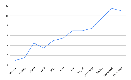
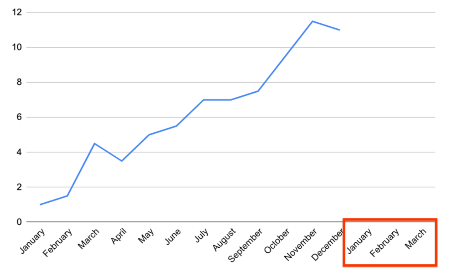
What Are We Predicting?

Sequence prediction aims to forecast future values based on historical data.

Example: Predicting the next quarter’s performance from a year of data.

Sequence prediction is about predicting what happens next in a sequence. For example, if we have a year’s worth of data, we may want to know what happens in Q1 of the next year.

RNNs for Sequence Prediction: A New Tool

• Traditional Approach: Statistical methods (e.g., ARIMA, Markov chains)
  • Often involve numerous assumptions.
    
• Machine Learning & RNNs: A largely non-parametric approach.
  • Data “speaks for itself,” fewer assumptions.
    
  • Requires more data for optimal performance.

The standard approach to sequence prediction for several years was a statistical one (like Markov chains or ARIMA).

There may not be a need to go into detail, but you could mention Markov Chains or ARIMA time series forecasting. Suffice to say, these approaches often require a lot of assumptions, such as a transition matrix of probabilities, or a normal distribution of noise.

RNNs allow the data to “speak for themselves.” Using an RNN is a largely non-parametric approach. The downside is that RNNs usually need more data to make good predictions.

Examples of Sequence Prediction

Walk students through the following examples. These are just a few examples. There are many more, so feel free to elaborate on these and/or add others.

Example: Stock Price Prediction

Predicting future stock prices based on historical market data.

A complex task due to market volatility, but RNNs can capture trends.

One of the most common examples of sequence prediction is predicting stock prices. Stock prices are notoriously volatile, but a lot of people are involved in the practice of trying to predict them. There are entire industries based on this practice.

Example: Weather Forecasting

Forecasting weather patterns based on past meteorological data.

While complex, RNNs can identify subtle temporal dependencies.

Predicting the weather based on previous days of weather could also be an important application of sequence prediction. While most meteorological systems use a parametric approach based on input data (such as air pressure, cloud cover, etc.), a sequence prediction model can go surprisingly far.

Example: Predicting Passenger Traffic

Predicting daily traveler numbers at a train station.

RNNs can learn seasonality (weekdays vs. weekends, holidays).

Requires sufficient historical data to capture these patterns.

You may want to predict the number of travelers at a train station on a given day, given the previous data of how many travelers were there each day. RNNs pick up on things like varieties of seasonality (e.g., weekday vs weekend, holiday season) and noise.

However, especially for time series with seasonality, we need to have enough data. For example, if we only have data for October and November, we won’t do very well at predicting December because it is a holiday month; we would ideally have data for December of the previous year (if not multiple years).

Your Turn: RNNs for Vibration Prediction

In the lab, you will use an RNN to predict a sequence of vibration readings from an engine.

You’ll apply TensorFlow with Keras to build, test, and tune your model.

In the lab we’ll use a recurrent neural network to predict a sequence of vibration readings from an engine. We’ll see how to apply TensorFlow with Keras to build, test, and tune your model.

Natural Language Processing (NLP)

What is Natural Language Processing?

The interaction between computers and human (natural) language.

Enables computers to understand, interpret, and generate human language.

So what is natural language processing?

What are some applications of NLP in your everyday life? Prompt the group to respond.

NLP Applications in Everyday Life

• Autocorrect & Predictive Text
  
• Translation Services (e.g., Google Translate)
  
• Parsing Text (e.g., extracting information)
  
• Chatbots & Virtual Assistants
  
• Question Answering Systems
  
• Speech Recognition

… and so much more!

Here are some examples of what is considered natural language processing. You have likely interacted with systems that perform these tasks before.

There is some argument regarding whether speech recognition should actually be considered NLP. It is possible to convert sound waves into words without actually understanding what those words are. This is technically “processing” of natural language, but it falls short of “Natural Language Understanding.” However, many speech recognition systems actually attempt to understand the speech in order to correctly predict ambiguous words like “there,” “their,” and “they’re.”

Character vs. Word-Level Models

Character-Level Models:
- Process text one character at a time.
- Can handle out-of-vocabulary words and typos.

Models can process text at different levels. For example, you’ll see some language generation models that use a character-by-character approach such as the RNN shown in this slide.

Character vs. Word-Level Models (Cont.)

Word-Level Models:
- Process text one word at a time.
- More common for English and similar languages.
- Often faster to train and perform well.

Which is better? Depends on the language and use case.

Here is a word-based model. It looks structurally like the character-based model except that it works at the word level.

Which is better?

It depends. For some languages and use cases, the character-based approach works well. In practice, you see more word-based models, especially for English and similar languages. The models typically perform well and are quicker to train than character-based models.

Text Processing: Regular Expressions (Regex)

A powerful tool for pattern matching in strings.

Used for extracting, validating, or modifying text.

regex	matches
[wW]ood	wood, Wood
beg.n	begin, begun, beg3n
o+h	oh, oooooh
[^a-zA-Z]	a single non-alpha character

Before machine learning, NLP problems were usually solved by pattern matching. Even now, these text processing techniques can be very important in processing messy natural language.

Regular expressions are widely used in text processing. Imagine needing to extract all the email addresses from a block of text or remove prefixes/suffixes from a word. A regex defines a pattern that is used to match certain character combinations, following a set of rules. In this table we show a few examples of pattern matching rules:
* “.” matches any single character
* “+” matches 1 or more of the previous character
* “[^...]” negates the rest of the pattern in the brackets

Regex rules can be very powerful but also very complex. Many guides exist for effectively using regexes: https://www.rexegg.com/regex-quickstart.html

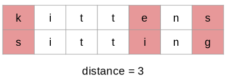
Text Processing: Minimum Edit Distance

Also known as Levenshtein distance.

• Measures the minimum number of single-character edits (insertions, deletions, substitutions) required to change one string into another.
  
• Crucial for autocorrect, spell checkers, and evaluating text generation systems.

Another important concept for text processing is minimum edit distance, also called Levenshtein distance. This is especially useful for autocorrect tools and evaluating systems that generate language, e.g., translation. There are many open source Python implementations of this metric that you can use.

Feature Extraction in NLP

Transforming raw text into informative numerical features.

• N-grams: Consider sequences of n words.
  • Captures context beyond single words (e.g., “not horrible”).
    
• TFIDF (Term Frequency-Inverse Document Frequency):
  • Determines word importance in a document.
    
  • Discounts common words like “the” or “and.”
    

Tip

N-grams help capture local word order, while TFIDF helps identify unique and important terms.

Before neural networks, the first step in NLP was “feature extraction,” or transforming raw text into informative features. The idea is that just the individual words in a text do not fully capture the meaning of the text.

One very common feature extraction technique is n-grams, which consider n-word sequences instead of just individual words. In the original sentence “that movie was not horrible,” the word “horrible” may cause a model to predict very strong negative emotion. But, if we extract bigrams (2-grams), then we would correctly pair “not horrible,” which is a much milder emotion.

Another common technique is TFIDF, which calculates how important a word is to a text. This often has the effect of ignoring more common words like “the” and letting the model focus on more unique words in the text.

Language Modeling: Bag-of-Words

Simplest language modeling approach.

Treats a sentence as an unordered collection of words.

Example: “I love love loved it!” and “I HATED it :-(”
- Meaning can often be inferred without word order.

To build models for NLP tasks, we must have some notion of how words fit together into sentences and text. Language modeling refers to determining how likely a certain sentence is. The simplest language modeling approach is a bag-of-words: treat a sentence like an unordered collection (set) of words.

Take an example movie review, “I love love loved it!”, and another, “I HATED it :-(”. As humans, we could deduce which review corresponded to a positive sentiment and which review corresponded to a negative sentiment, even if we looked at these sentences out of order (e.g., “it! I loved love love” and “HATED :-( I it”). So bag-of-words is like saying, “I’m pretty sure I can glean the meaning of sentences, with words in any order, so why bother keeping track of the order? Sounds like more work to me.”

But can you think of an example or two where this strategy would fail? Especially consider if you’re trying to predict more than just two sentiments (“good” and “bad”). Prompt class for discussion.

Language Modeling: Sequential Words

While bag-of-words is effective for some tasks (e.g., spam filtering), word order is crucial for complex NLP.

Sequential approaches preserve word order.

This is where Recurrent Neural Networks (RNNs) become indispensable.

Bag-of-words approaches are surprisingly successful on many tasks (email spam filter, sentiment analysis) and are less computationally intensive.

But fundamentally we know that the order of words matters. Harder NLP tasks build upon sequential approaches, which preserve the order of words in a text. This is exactly what RNNs are useful for. Recurrent Neural Networks handle this well.

The NLP Processing Pipeline

Understanding the typical flow for NLP tasks:

graph TD
    A["Raw Text"] --> B{"Feature Extraction / Embeddings"};
    B --> C["Machine Learning Model"];
    C --> D["Supervised Task (e.g., Classification, Generation)"];

The typical process for an NLP task is:
1. Raw text
2. Transform to feature vectors (either through feature extraction or embeddings)
3. Run through some model
4. Perform supervised task

Your Turn: NLP Lab

In the lab, you will perform sentiment analysis on reviews.

You will then build a classifier to determine authorship (e.g., Jane Austen vs. Charles Dickens).

In this lab we will perform sentiment analysis on reviews as an example. After that we’ll write a classifier that determines if a piece of text was written by Jane Austen or Charles Dickens.

Conclusion and Q&A

We’ve explored Convolutional Neural Networks for image processing, Recurrent Neural Networks for sequential data, and key concepts in Natural Language Processing.

These deep learning techniques are fundamental to many modern ECE applications.

What questions do you have about these powerful tools and their applications in engineering?