Machine Learning

04 Classification: Image Classification & Processing

Imron Rosyadi

05. Introduction to Image Classification

We’ll explore how machine learning tackles visual data, understanding its unique challenges and opportunities for ECE applications.

We have performed binary and multiclass classification on datasets containing string and numeric values. In this unit we’ll perform classification on images. This transition from abstract data to concrete visual information is crucial for many ECE applications.

The Nature of Image Features

What makes image classification unique? Each pixel is a feature, represented by numerical values.

Pixel Grid Representation

What makes image classification different from other forms of classification? One major difference is the features. When classifying an image, each pixel is a feature. How are these pixels represented? Understanding this representation is fundamental for ECE students to grasp data acquisition and processing.

RGB Pixel Values

Pixels are often encoded using Red, Green, and Blue (RGB) values. Each color component typically ranges from 0 to 255.

RGB Color Model

Often pixels are represented as RGB values. These are three numbers that indicate the amount of red, green, and blue in an image. These numbers often range from 0 to 255. This multi-channel representation is key for color images, but it significantly increases feature dimensionality.

Feature Dimensions: A Challenge

Consider a 1920 × 1920 image. How many features if represented by RGB values?

Let’s take a moment to think about the number of features we are dealing with there. Say we have a 1920 by 1920 pixel image. How many features would we have? This calculation highlights the computational burden of raw pixel data.

Feature Dimensions: The Calculation

\[ 1920 \times 1920 \times 3 = 11,059,200 \]

That’s over 11 million input features! Data can be viewed as a 3D tensor: Width × Height × Channels.

That’s over 11 million input features! This is an enormous number for a standard machine learning model to handle directly. We can think of the data as a 3-d matrix (or a tensor) with dimensions 1920 x 1920 x 3.

Interactive Feature Calculator

Explore how image dimensions and color channels impact the total number of features.

viewof image_width = Inputs.range([10, 2000], {value: 1920, step: 10, label: "Image Width (pixels):"});
viewof image_height = Inputs.range([10, 2000], {value: 1920, step: 10, label: "Image Height (pixels):"});
viewof color_channels = Inputs.select(["1 (Grayscale)", "3 (RGB/BGR)", "4 (RGBA/BGRA)"], {value: "3 (RGB/BGR)", label: "Color Channels:"});

Note

Adjust the sliders and dropdown to see the feature count change dynamically!

This interactive calculator helps visualize the scale of image data. Students can play with different resolutions and channel counts to directly observe the explosion of features. This ties into computational complexity and hardware considerations in ECE.

Even More Features

How many features would a 12 megapixel image (common for phone cameras) have if stored in RGB?

Let’s try another one. How many features would we have for a a 12 megapixel image stored in RGB? This resolution (or greater) is common for mobile phones these days. This is a practical example of real-world image sizes.

Megapixel Feature Count

\[ 12,000,000 \times 3 = 36,000,000 \]

An extremely large number of features! This makes training traditional models difficult. Lower resolution images are often used for initial training.

This is an insanely huge number of features. It is extremely difficult for a model to perform well with such a huge number of features directly. That is why you’ll notice that the images we use in this lab are very low resolution. This also motivates the need for specialized architectures like Convolutional Neural Networks (CNNs) that can handle such high dimensionality efficiently.

Grayscale: Reducing Complexity

Grayscale images use a single number (e.g., 0-255 or 0.0-1.0) to represent pixel intensity. This effectively reduces the feature count by a factor of three.

Grayscale Image

Another way to reduce the number of features is to convert them to grayscale. Grayscale uses a single number to represent the intensity of color in a pixel, but it doesn’t specify the color. The range of values that you’ll find vary. In this lab we work with one dataset that has a grayscale range of 0 through 255 and another that goes from 0 through 16. Grayscale values might even be in the range from 0.0 through 1.0. For neural networks this smaller range is easier to train on and aids in faster convergence.

Other Image Formats

Beyond RGB and Grayscale, various formats exist, each with specific applications:

• HSV: Hue, Saturation, Value (perceptually organized)
• HSL: Hue, Saturation, Light (perceptually organized)
• CMYK: Cyan, Magenta, Yellow, Black (for printing)
• BGR: Blue, Green, Red (common in some computer vision libraries)

There are more color models than RGB and grayscale. A few alternatives are listed in this slide. You’ll notice that some, like CMYK, have more values than RGB. BGR, on the other hand, is just RGB in a different order. Understanding these alternatives is important for ECE students who might work with cameras, displays, or different image processing pipelines.

Real-World Image Challenges

Images encountered in real-world scenarios are rarely simple. They often contain multiple objects and background clutter.

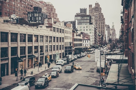
Busy Street Scene

Another interesting aspect of image classification is that images rarely contain just a single item. Take this image, for instance. It contains buildings, cars, people, and more. With an image like this, it can be hard for the model to identify the important features. Sometimes this requires the researcher to pre-process and clean the images. Sometimes it requires additional model tuning. This is where ECE expertise in signal processing and intelligent systems becomes critical.

Lab Exercise: Fashion-MNIST

We’ll start with controlled datasets, like Fashion-MNIST: 70,000 grayscale, 28x28 pixel images of single clothing items.

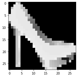
Ankle Boot Example

In the lab for this unit, we’ll work with some very curated datasets. The first dataset we’ll work with is the Fashion-MNIST dataset. The dataset contains 70,000 images of different clothing items. Each image is a grayscale image, only contains one item, and is only 28x28 pixels. This low-resolution and curated nature allows us to focus on the classification task without overwhelming computational resources.

Fashion-MNIST Class Labels

Label	Class
0	T-shirt/top
1	Trouser
2	Pullover
3	Dress
4	Coat
5	Sandal
6	Shirt
7	Sneaker
8	Bag
9	Ankle boot

The images in the Fashion-MNIST dataset are labeled with one of the shown classes. The numeric label is the target of the model. This is a multi-class classification problem.

Lab Exercise: MNIST Digits

Another clean dataset: handwritten digits for classification (0-9). Similar 28x28 grayscale format, one digit per image.

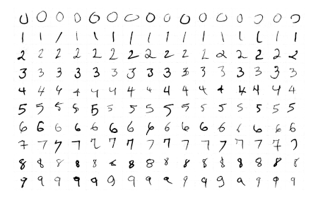
Handwritten Digits

We’ll also work with the MNIST digits dataset. This dataset contains handwritten digits that we’ll classify as 0 through 9. This is also a very clean dataset with one digit per image. Both Fashion-MNIST and MNIST are benchmarks in machine learning for image classification, ideal for introductory labs.

Your Turn!

Get hands-on experience with image classification datasets.

06. Images and Videos

Images and video processing are integral to many ML applications in ECE.

In this unit we will move away from machine learning for a bit and instead talk about images and videos. Why images and videos? Image and video processing is actually very common in machine learning applications. Can you think of any examples of images or video processing in machine learning? Some ideas include: facial recognition, classification, converting video to a textual description (story), analyzing video for suspicious movements, disease detection in medical images, crop yield estimates based on aerial photos of fields. The list goes on and on. There are many applications of image and video processing in machine learnings, especially relevant for ECE fields like robotics, embedded systems, and computer vision.

What is an Image, Really?

At its core, an image is a grid of pixels. Each pixel is a sampled data point representing color at a specific location.

Let’s think for a second. What is an image actually? You likely know that an image is a grid of pixels. And each pixel represents a single color point in the image. But how is that pixel encoded? From an ECE perspective, this means understanding analog-to-digital conversion and spatial sampling.

Image Encodings

Not all pixels are encoded in the same way. Various encoding schemes exist, influencing data representation and processing.

Not all pixels are encoded in the same way. There are actually quite a few different encodings for images. Choosing the right encoding can significantly impact memory usage, processing speed, and model performance.

Grayscale vs. Color Images

A primary distinction: single-channel grayscale or multi-channel color. This choice affects feature count and information richness.

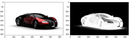
Color vs Grayscale Car

One of the first distinctions to be made is if the image is made up pixels on a “gray scale” or if the image is made from a larger spectrum of colors. In this example you can see that the image on the left has many colors, including some reds while the image on the right is limited to black, white, and the grays in between. What does this mean for the encoding? This decision impacts the computational load and the type of features a model can extract.

Grayscale Pixel Ranges

Grayscale values can range from: - Integers: [0, 255] (8-bit unsigned integer) - Floats: [0.0, 1.0] (normalized for neural networks)

Grayscale Car

We’ll start with the simplest format, grayscale. Grayscale images have a single numeric value representing each pixel in the image. But what are those numbers? Typically they range from 0 to 255 if they are integers or 0.0 to 1.0 if they are floating point values. Even with grayscale images, it is important to know the range of values for the input pixels. If the pixels range from 0.0 to 1.0 then many models will be able to more easily train on the images due to better gradient flow properties. If the values are integers between 0 and 255, then it is typically a good idea to divide the values by 255.0 in order to bring them into the 0.0 to 1.0 range that neural networks prefer to help models learn more quickly. This normalization is a common pre-processing step in ECE ML applications.

Interactive Pixel Normalizer

Normalize a pixel value from [0, 255] to [0.0, 1.0] or vice versa.

viewof pixel_value_0_255 = Inputs.range([0, 255], {value: 128, step: 1, label: "Input Pixel Value (0-255):"});
viewof normalization_type = Inputs.select(["Normalize to [0.0, 1.0]", "Scale to [0, 255] (from [0.0, 1.0])"], {value: "Normalize to [0.0, 1.0]", label: "Operation:"});

Demonstrating pixel normalization is vital for ECE students. It shows how raw sensor data (e.g., 0-255 from an ADC) is often transformed into a range amenable to neural network training, which is typically floating-point values between 0 and 1. This interactive element allows them to see the direct mapping.

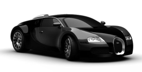
Color Image Encodings: A Spectrum

From RGB to CMYK, many color spaces exist. Each offers a different way to represent color, impacting applications from display technology to printing.

Color Car

Grayscale images typically are one of the two encodings that we mentioned. It is of course important to know which encoding your images are in since a model expects inputs to be on the same scale. However, converting between [0.0, 1.0] and [0, 255] is fairly trivial. Color images introduce an entirely new level of encoding complexity. There are scores of encodings for color images. One of the more common ones that you might have seen is RGB. RGB stands for “red”, “green”, “blue”. With these three colors you can make scores of other colors. With RGB encoding a value, typically between 0 and 255 (though sometimes between 0.0 and 1.0), you can combine the colors to create a rainbow of possibility. With RGB you have three numeric values for each pixel. This triples the size of your inputs! But that is not all. There is RGBA, which takes our red, green, and blue and adds an “alpha” channel which represents the opacity of the pixel. Opacity? Typically when we think of an image, we think about only seeing that image. But what if we put an image under the image we were looking at? If there were no opacity, then we’d only see the topmost image. If there is opacity (think transparency) then we would see a little bit of the underlying image too. The alpha channel, also typically between 0 and 255 or 0.0 and 1.0, manages how “see-through” our pixel is. But why RGB? Why not BRG or GBR or any other ordering? It turns out that there are other orderings, one of the more common being BGR. This was a common encoding in early digital cameras for hardware reasons that aren’t relevant to our topic. Just know that color order can change, and you need to make sure that your inputs for training and predicting have the same encodings. Of course, this begs the question. Are reds, greens, blues, and maybe alphas the only way to encode color? Of course not! There are other schemes such as CMYK, which stands for cyan, magenta, yellow, and black. Encodings aren’t complicated individually, but the number and variety of image encodings can be difficult to work with. Know your inputs!

Modifying Images: Encoding Transformations

Python libraries like OpenCV (cv) and NumPy (for array operations) facilitate these transformations.

import cv2

# Convert from BGR encoding (common in OpenCV) to RGB 
image = cv2.cvtColor(image, cv2.COLOR_BGR2RGB)

# Normalize pixel values from [0, 255] to [0.0, 1.0]
image = image / 255.0

# Scale pixel values from [0.0, 1.0] back to [0, 255]
image = (image * 255).astype(int) 

We talked about image encodings and how it is important to feed your model images encoded in the same way. In order to do this you have a few options. If you are converting encodings, you can use the OpenCV cvtColor function to do the conversion for you. If you are scaling the encodings you can use simple Python expressions with NumPy arrays. These are standard operations in many ECE signal processing pipelines.

Modifying Images: Resizing

Resizing images is often necessary to match model input requirements. Care must be taken to avoid distortion.

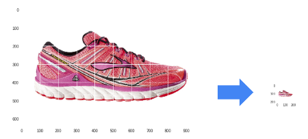
Resized Running Shoe

But what about scaling/resizing an image? Some models have a scaling layer as an early step, but not all do. Also, you may want more control of your image when you scale it. In the example in this slide we simply scaled the image down to a size that presumptively the model expects. We could have also padded it into a proportional square or rectangle before resizing. Resizing algorithms can involve various interpolation methods (e.g., nearest-neighbor, bilinear, bicubic), which are key considerations in image processing.

Modifying Images: Padding

Padding helps maintain aspect ratio and prevents image distortion during resizing. Useful for ensuring all images conform to a fixed input size.

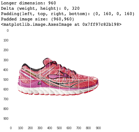
Padded Running Shoe

But you don’t always just want to blindly resize an image. That might distort it. In some cases you’ll want to pad an image with whatever the background color is and then resize it in order to avoid distorting the image. To do this, you must find the number of pixels to add to the height of the image and divide those pixels across the top and bottom of the image. You must do the same for the left and right of the image. This is a common pre-processing technique, especially in image recognition with CNNs.

Modifying Images: Centering

Advanced techniques can find and center the focal object. Algorithms like Canny edge detection help pinpoint important features.

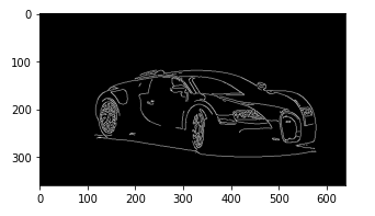
Car with Edge Detection Lines

If we have images with a predictable solid background, we can actually perform more complex processing and try to find the center of the focal object. Using algorithms like the Canny algorithm, we can find the key strokes and make our image, hone in on them, and find the center of our image. We can then pad around that. This involves control systems and image analysis, direct applications for ECE students.

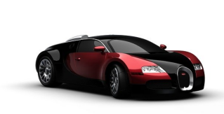
Modifying Images: Rotation

Image augmentation often involves various transformations, including rotation, to increase data diversity and model robustness.

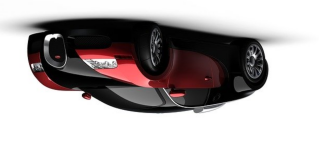
Rotated Color Car

Other image manipulation tricks involve rotations. You can augment an image by spinning it around. Data augmentation like rotation helps improve model generalization by exposing it to varied orientations of objects without needing more real-world data.

Other Image Augmentations

What other image augmentations can you imagine?

• Cutting/Mixup: Splicing parts of images to create new training examples.
• Dropout: Randomly removing portions of an image during training.
• Generative Models: Creating synthetic data to augment existing datasets.
• Color Jittering: Randomly adjusting brightness, contrast, saturation.

What are some other image augmentations that you can think of? Some others include: ‘cutting’: where images of the same class are spliced together to increase the size of the training data set. ‘drop out’: where portions of training images are removed during training. Generating fake data based from a model that is then used to train another model. There are many more strategies and none are right for every model. You have to experiment. Data augmentation is a powerful technique to prevent overfitting and improve model performance in data-scarce scenarios, a critical aspect of practical ML deployment in ECE systems.

Understanding Video Data

For our purposes, video is simply a sequence of images (frames).

Consider:

• Frame Rate (FPS): Number of images per second (e.g., 30 fps, 60 fps).
• Change between frames: Varies greatly based on content.

This section also talks about video. We are going to greatly simplify video. If you think about a video feed, it has images, it has sound, it might have captions and other optional features. For our case in this course, video will simply be a series of images and we will treat it as such. Much of the video we watch is 30 “frames per second” (fps) or 60 fps. Think of each of these frames as a still image. Now think about how much changes between frames in 1/30th of a second? Well, it depends on what type of video you are processing. Are you watching the spray from a sneeze? Are you watching ice melt? Video might simply be a “series of images” for our purposes, but you still need to consider what you are modelling. This understanding is key for ECE applications in real-time video processing, such as autonomous vehicles or surveillance.

Your Turn

It’s time to practice working with images and video.

This involves multiple labs:

1. Image processing with PIL (Pillow).
2. Image processing with OpenCV.
3. Video processing (extracting frames from video).

These labs build towards a project on classifying items in a video. Have fun!

07. Saving and Loading Models

In real-world applications, models are typically saved after training and loaded for deployment.

This enables reusability, fine-tuning, and sharing.

So far in this course, we have built models and used them immediately. In practice, you’ll find that you need to save your models and load them for use later. You’ll also find models published online that you can load and start using immediately or use as a warm start for training your own model. This concept of model lifecycle management is crucial for ECE engineers deploying ML solutions on embedded systems or cloud platforms.

Pickling scikit-learn Models

Standard Python’s pickle module can serialize (save) and deserialize (load) scikit-learn models.

Saving a model

import pickle
from sklearn.linear_model import LogisticRegression
# Assume 'model' is a trained scikit-learn model
model = LogisticRegression() # Placeholder for a real trained model
# ... train model ...

model_file = 'my_model.pkl'

with open(model_file, 'wb') as output:
    pickle.dump(model, output, pickle.HIGHEST_PROTOCOL)

Loading and using a model

import pickle
model_file = 'my_model.pkl'

with open(model_file, 'rb') as input:
    model_restored = pickle.load(input)

# Example: make a prediction (dummy input)
print(model_restored.predict([[45, 34, 2]])) # Placeholder

For models created using scikit-learn, we can use standard Python pickling to persist and reload the model. pickle.HIGHEST_PROTOCOL ensures compatibility and efficiency. This method is straightforward for simpler models, but attention to library versions is important for compatibility.

Saving and Loading Keras Models

Keras (built on TensorFlow) provides native functions for saving and loading models in its own format or H5.

Saving a Keras model

import tensorflow as tf
from tensorflow import keras
# Assume 'model' is a trained Keras model
model = keras.Sequential([keras.layers.Dense(1, input_shape=(3,))]) # Placeholder

tf.keras.models.save_model(
    model, 'my_model.tf'
)

Loading a Keras model

import tensorflow as tf

loaded_model = tf.keras.models.load_model(
    'my_model.tf'
)
# Example: Summarize the loaded model
loaded_model.summary()

Keras-based models can be saved and loaded using the save_model and load_model functions. By default the models are in a TensorFlow-specific format, which is optimized for TensorFlow’s execution graphs. However, the models can also be saved as H5, which is another popular file format for storing models, often more portable. This is particularly relevant for ECE engineers deploying Keras models on various hardware accelerators.

Loading Frozen Graphs: Historical Context

“Frozen graphs” refer to TensorFlow 1.x models saved as a single .pb file. They represent a static computation graph with embedded weights.

Loading the Graph Definition

import tensorflow as tf
import os

frozen_graph_path = os.path.join("path", 'frozen_inference_graph.pb')

with tf.io.gfile.GFile(frozen_graph_path, "rb") as f:
    graph_def = tf.compat.v1.GraphDef()
    loaded = graph_def.ParseFromString(f.read())

Note

This process uses tf.compat.v1, indicating compatibility for older TensorFlow 1.x models within a TensorFlow 2.x environment.

There is also the concept of freezing graphs. Some models, such as the one we’re going to use in this lab and in our next project, are distributed in this manner. In order to “unfreeze” a graph, you must first load the graph into a GraphDef object. Notice that this is using a TensorFlow version 1 compatibility layer object. This process is useful for loading models built in TensorFlow version 1, which many legacy systems in ECE might still use.

Loading Frozen Graphs: Wrapping for TF2

TensorFlow 1.x used lazy execution; TensorFlow 2.x uses eager execution. tf.compat.v1.wrap_function bridges this gap for seamless integration.

def wrap_graph(graph_def, inputs, outputs, print_graph=False):
    wrapped = tf.compat.v1.wrap_function(
        lambda: tf.compat.v1.import_graph_def(graph_def, name=""), [])

    # Prune the graph to only include specified inputs and outputs
    return wrapped.prune(
        tf.nest.map_structure(wrapped.graph.as_graph_element, inputs),
        tf.nest.map_structure(wrapped.graph.as_graph_element, outputs))
  
# Example usage:
model = wrap_graph(graph_def=graph_def,
                   inputs=["image_tensor:0"], # Name of the input tensor
                   outputs=["detection_boxes:0", "detection_scores:0"]) # Example output tensors

The programming models of TensorFlow 1 and 2 are quite a bit different. TensorFlow 1 used lazy execution (defining the graph first, executing later) while TensorFlow 2 uses eager execution (operations execute immediately). In order to bridge the gap in these execution models, we need to wrap our TensorFlow version 1 graph. This wrapping makes the TF1 graph behave like a TF2 callable function, simplifying its use in modern workflows. This is a common challenge for ECE engineers maintaining or upgrading ML infrastructure.

Loading Frozen Graphs: Using the Wrapped Model

Once wrapped, the frozen graph can be used like any other TensorFlow 2.x callable.

# Assuming 'tensor' is a pre-processed image tensor
predictions = model(tensor) 

# 'predictions' would contain the outputs defined earlier, e.g.,
# predictions["detection_boxes:0"], predictions["detection_scores:0"]

And now we can use the model as a function. We pass it in tensor objects and get predictions back. This demonstrates how backward compatibility is handled, enabling ECE professionals to leverage older, pre-trained models.

Your Turn

Practice saving and loading models using different frameworks to understand their practical deployment.

08. Video Processing Project: Identifying Cars in a Video

Combine image processing, pre-trained models, and video manipulation to perform object detection in real-time video.

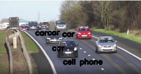
Cars with Bounding Boxes

We are about to combine many of the skills we’ve learned over the past few units. We will take a video file and a pre-trained model and build bounding boxes around items in each frame of the video. This is a complex project directly applicable to ECE fields like autonomous vehicles, traffic monitoring, and surveillance systems.

Review: Image Data Representation

How is image data typically represented and stored? What are the features?

Exercise (5 minutes) Have students discuss the fact that images are simply pixels. There are different ways to represent pixels, but it’s common to use RGB values that each range from 0 to 255. Each pixel is a feature. Remind them that image data can be challenging to work with because it is often very large. For example, a 12 megapixel image has 36,000,000 features. You may mention that grayscale is one way to cut down on the number of features. This review reinforces the foundational concepts before tackling the project.

Review: Python Libraries for Image/Video

What Python libraries have we used for image and video manipulation?

Exercise (5 minutes) Have students discuss the labs they completed using PIL (Pillow) and OpenCV. These are industry-standard libraries, and knowing their application is crucial for ECE students in computer vision.

Review: Classification with Image Data

How have you performed classification tasks with image data?

Exercise (5 minutes) Have students discuss the fact that they used TensorFlow to train a simple classification model for the Fashion MNIST dataset. This was a prefabricated dataset that was relatively small, so it was possible to train a simple model locally and in a reasonable amount of time. For larger classification tasks, we discussed using pre-built models (specifically those stored in the TensorFlow detection model zoo). This connects past labs to the current project and future complex applications.

Video Processing Project Overview

Process video frame-by-frame, applying a pre-trained object detection model. Visualize detections by drawing bounding boxes around identified objects.

Video Frame with Bounding Boxes

Now let’s talk about the project for today! Here you can see a single frame of a video showing a road with a bunch of cars. A machine learning model, like the one you will use, has identified many of the cars in the image and labeled them as “car.” One was strangely labeled as a cell phone. Clearly models are not perfect. In this project we will process a video frame-by-frame and create bounding boxes around items found in those images by the third-party model. This real-world scenario demonstrates the power and limitations of current ML models.

Your Turn

This lab will exercise many of your Python and modeling skills. Let’s get started!

09. Classification Gone Wrong

Even the most sophisticated models can make mistakes or exhibit biases. Understanding these failures is as important as understanding successes.

Note to facilitator: This is an activity best used during the Classification lessons in Track 4. It focuses on small group discussions and involves limited setup and facilitation by the instructor. It would best be taught in about 35 minutes, but it could be stretched to 45 minutes depending on the number of groups and how long you want to allow for discussion. This section emphasizes ethical considerations in ML, crucial for ECE students developing responsible AI systems.

What Do You See First?

Perception can be ambiguous. Similarly, ML models can misinterpret data, leading to serious issues.

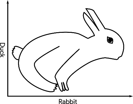
Duck-Rabbit Ambiguous Illusion

When you look at this, what do you see first? Raise your hand if it’s a duck you see first. Raise your hand if it’s a rabbit you see first. You’ve likely seen similar ambiguous images, images where one thing jumps out at you at first, and it takes a little longer to see something else. This phenomenon is likely based on humans and their individual schemas. But models can make the same kinds of errors, which can lead to some serious issues. Today we’ll discuss three separate scenarios of classifications that did not go as planned and the impact they caused.

Framing Harmful Classifications

• Often, bias is unintentional, not malicious.
• However, errors can be difficult to fix once deployed.
• Mistakes can have long-lasting, negative repercussions on individuals or groups.

Most people don’t set out to make a harmful or biased system; they set out to create a model that does one thing, but it ends up having other effects that could be unintended. This happens frequently. You can search for many, many examples of machine learning projects gone awry, some more serious than others. When these mistakes occur, they’re often very difficult to remedy because they require collecting new data, retraining a model, etc. If your dataset was biased to begin with, then focusing your data collection on only one type of data to remedy your initial issue may lead to another type of bias. These mistakes can have a negative and far-reaching impact on people or entire groups. Understanding the societal impact of ML is an ethical imperative for ECE professionals.

Group Activity

Divide into groups (1, 2, 3) and each read a corresponding article. Be prepared to discuss the implications of “classification gone wrong.”

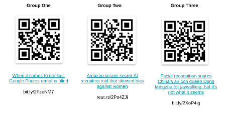
Group Collaboration Image

Let’s break into groups by counting off 1, 2, and 3. Group 1, you will read the corresponding article. The same goes for groups 2 and 3.

Group Discussion Prompts

1. Read the article as a group (10 minutes).
2. Discuss the following questions (15 minutes):
   • What was the original intent of this model/system?
   • Describe the bias with the model that led to this problem.
   • What was the cause of this problem?
   • Are there other mistakes that this model/system could make with this same root problem?
   • What are the short-term and long-term impacts of this?
3. Each group will present to the class (5 minutes/group).

Each group will read their article and discuss these questions. After reading and your group discussion, each group will present to the class. You may have one member of your group present or several. When planning this 5-minute presentation, please allow one minute for questions. Give students a 5-minute warning to begin building a short presentation for the rest of the class. You can give students easel boards or posters to use as an aid to present or have them just use notes to verbally present. This encourages critical thinking and ethical analysis, vital skills for ECE graduates.

Class Discussion

• What was most surprising or alarming about these examples of bias?
• How can situations like this be prevented in future ML system designs?
• What is the real-world impact of these mistakes?
• What does this mean regarding your responsibility as professionals in ECE ML?

Note: If time permits, open up the discussion to the entire class after each group has presented. Encourage more follow-up questions and/or reflections of the questions listed on the slide. This final discussion brings together the ethical and technical aspects of ML, preparing ECE students for real-world challenges.