graph TD
    A[Start] --> B{Data Input};
    B --> C[Predict Target];
    C --> D[Compare to Actual Target];
    D --> E[Calculate Error/Loss];
    E --> F["Update Model Parameters <br> (Weights & Bias)"];
    F --> G{Stopping Condition Met?};
    G -- No --> C;
    G -- Yes --> H[Model Converged];
Machine Learning
03 Regression: Fundamentals, Implementation, and Evaluation
Regression

Regression Introduction Image
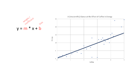
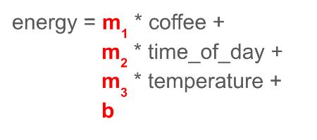
Mathematical Model
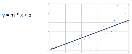
Mathematical Model for Linear Regression
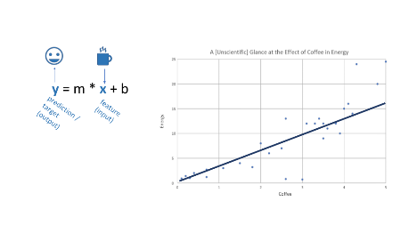
Features Go In, Targets Come Out
Features and Targets in Machine Learning
What is the Machine “Learning?”
Weights and Biases in Linear Regression
Multiple Features
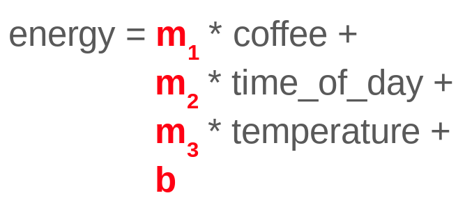
Multiple Features in Regression
Predict the Selling Price of a House
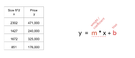
House Price Data
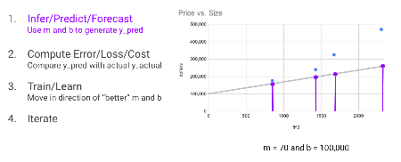
Predict the Price of a House Using the Machine Learning Process
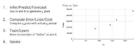
House Price Scatter Plot
Predict the Price of a House Using the Machine Learning Process
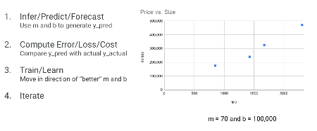
Initial Guess for Line
Predict the Price of a House Using the Machine Learning Process
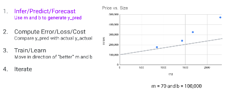
Line from Initial Guess
Predict the Price of a House Using the Machine Learning Process
Predicted Values Example
Predict the Price of a House Using the Machine Learning Process
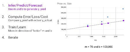
Actual vs Forecasted Values
Predict the Price of a House Using the Machine Learning Process
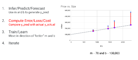
Error Calculation Illustration
Predict the Price of a House Using the Machine Learning Process
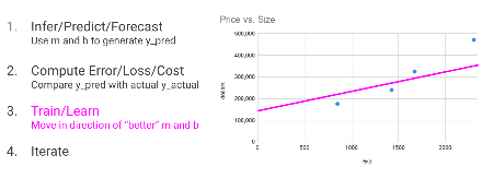
Updated Line Illustration
Error/Loss/Cost Functions
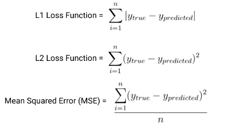
Common Loss Functions
Housing Example
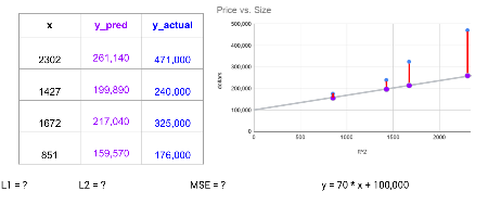
Housing Example Data Table
Housing Example (L1 Loss)
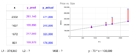
L1 Loss Calculation
Housing Example (L2 Loss)
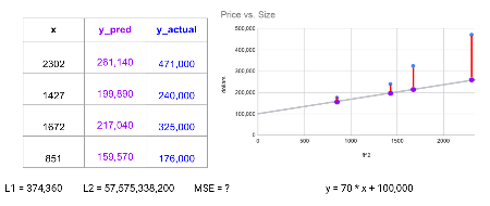
L2 Loss Calculation
Housing Example (MSE)
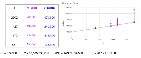
MSE Calculation
Gradient Descent
Gradient Descent Illustration
Linear Algebra Notation for \(y=mx+b\)
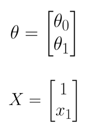
Linear Algebra Notation for Single Feature
Linear Algebra Notation for \(y=mx+b\)
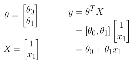
Compact Linear Algebra Notation
Multiple Regression (i.e. Multiple Features)
Multiple Features in Multiple Regression
Multiple Regression Notation
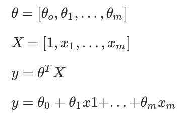
Multiple Regression Compact Notation
Batched Data
Break data into smaller batches.
- We’ll use a new batch on each learning step.
- New hyperparameter batch size controls how much data is used for each learning step.
Batched Data for Training
Hyperparameters We Care About
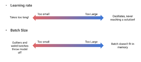
Hyperparameter Tuning Guidelines
Linear Regression

Linear Regression Fit Animation
Train/Validate, Test
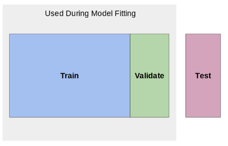
Train, Validate, Test Split
Train/Validate, Test, Validate
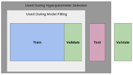
Double Validation Process
Predicted vs. Actual Plots
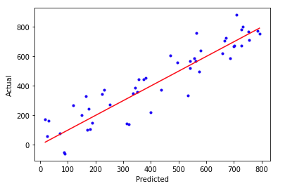
Good Predicted vs Actual Plot
Predicted vs. Actual Plots (Positive Bias)
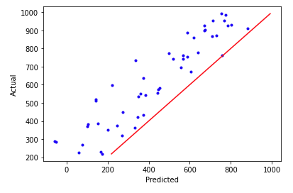
Predicted vs Actual Plot with Positive Bias
Residual Plots
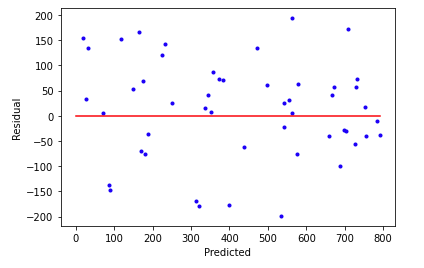
Good Residual Plot
Residual Plots (Bias Example)
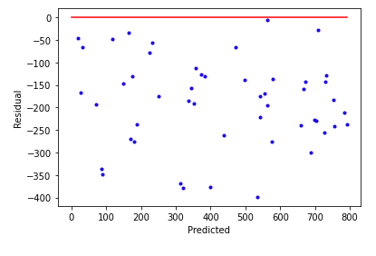
Residual Plot with Bias
Linear Regression Fit Animation
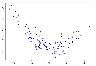
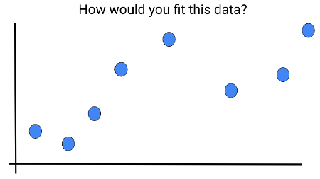
Dataset for Polynomial Regression
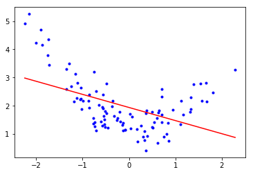
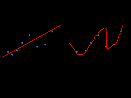
Linear Fit on Non-linear Data
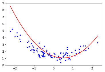
Polynomial Fit on Non-linear Data
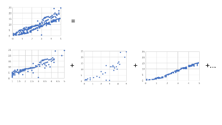
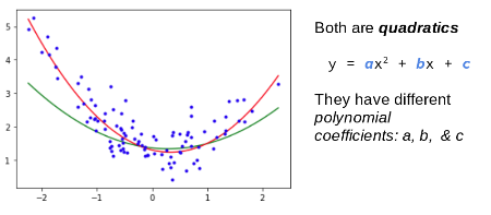
Polynomial Equations
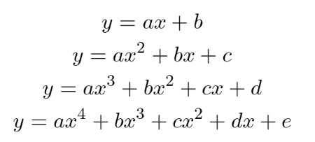
Examples of Polynomial Equations
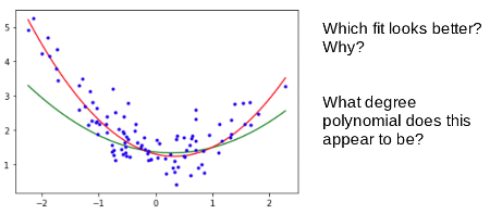
What is the Original Curve?
Original Polynomial Curve
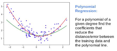
Polynomial Regression Process
Dataset for Overfitting Example
Overfitting Demonstration
Overfitting Analogy: Clothing Fit

Well-fitting shirt

Overfitted clothing

Underfitted clothing

Just right fit
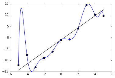
Illustration of Overfitting Regression
Recall: Mean Squared Error
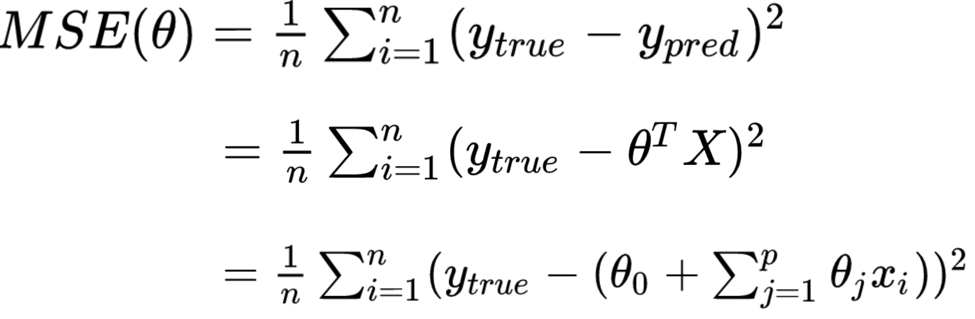
Mean Squared Error Formula Breakdown
Lasso (L1) Regularization
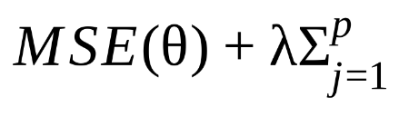
Lasso (L1) Regularization Formula
Ridge (L2) Regularization
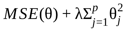
Ridge (L2) Regularization Formula