Motion, Pressure, and Flow Sensors
Instruments 5.2
Motion: From Position to Acceleration
If an object’s position is \(x(t)\) :
If we know acceleration \(a(t)\) , we can integrate to get:
Velocity : \[v(t) = v(0) + \int_0^t a(\tau)\, d\tau \tag{18}\]
Position : \[x(t) = x(0) + \int_0^t v(\tau)\, d\tau \tag{19}\]
An accelerometer measures \(a(t)\) \(v(t)\) \(x(t)\)
Stress that accelerometers only measure acceleration directly.
Velocity and position are reconstructed numerically or with analog integrators. This is exactly what is happening inside an IMU module used in robotics or phone motion tracking (plus sensor fusion with gyros and GPS).
Units & “g”
Proper SI acceleration unit: \(\mathrm{m/s^2}\)
Velocity: \(\mathrm{m/s}\)
Position: m
Often accelerations are normalized to earth gravity :
\(1\ \mathbf{g} \approx 9.8\ \mathrm{m/s^2}\)
So:
\(a = 2\ \mathbf{g} \Rightarrow a \approx 19.6\ \mathrm{m/s^2}\) Smartphone accelerometers will read roughly \(+1\ \mathbf{g}\) “down”
Point out the everyday experience: a car launch that “pins you to the seat” is well under \(1\ \mathbf{g}\) for most consumer cars.
Also mention that many MEMS accelerometers are specified directly in g (e.g., range ±2 g, ±16 g).
Vibration Motion Model
For simple periodic (harmonic) vibration:
\[
x(t) = x_0 \sin(\omega t) \tag{20}
\]
Where:
\(x(t)\) = position (m)\(x_0\) = peak displacement from equilibrium (m)\(\omega\) = angular frequency (rad/s)
Relationship between frequency and angular frequency:
\[
\omega = 2\pi f \tag{21}
\]
Emphasize: \(f\) (Hz) is cycles per second; \(\omega\) (rad/s) is radians per second.
This same sinusoidal model is used throughout ECE: AC circuits, signals and systems, vibrations, and controls.
Vibration: Velocity & Acceleration
Starting with \[x(t) = x_0 \sin(\omega t)\]
Velocity (first derivative):
\[
v(t) = \omega x_0 \cos(\omega t) \tag{22}
\]
Acceleration (second derivative):
\[
a(t) = -\omega^2 x_0 \sin(\omega t) \tag{23}
\]
All three signals are sinusoids at the same frequency .
They differ by amplitude and phase .
Peak acceleration:
\[
a_{\text{peak}} = \omega^2 x_0 \tag{24}
\]
Peak acceleration rises with \(\omega^2\) quadruples peak acceleration (for the same displacement).
This is why high‑frequency vibration can be extremely destructive, even for tiny displacements.
Make the connection to fatigue in mechanical structures, PCB vibration failure, etc.
Spring–Mass Accelerometer Principle
Core idea: combine Newton’s law and Hooke’s law .
Newton: \(F = ma\)
Hooke: \(F = k \Delta x\)
Equate forces:
\[
ma = k\Delta x \tag{25}
\]
Solve for acceleration:
\[
a = \frac{k}{m} \Delta x \tag{26}
\]
So:
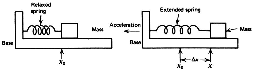
A test mass (seismic mass) attached to a spring is accelerated.
The mass “lags” behind slightly, stretching/compressing the spring by \(\Delta x\) .
Measure \(\Delta x\) → infer \(a\) .
Reinforce:
Many accelerometer designs differ only in how they measure \(\Delta x\) (potentiometer, LVDT, capacitive, piezoelectric, etc.).
MEMS accelerometers use tiny silicon springs and measure displacement capacitively.
Natural Frequency & Damping
Any mass–spring system has a natural frequency \(f_N\) :
\[
f_N = \frac{1}{2\pi} \sqrt{\frac{k}{m}} \tag{27}
\]
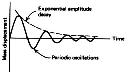
And a damped transient response after a disturbance:
\[
X_T(t) = X_0 e^{-\alpha t} \sin(2\pi f_N t) \tag{28}
\]
Where:
\(X_T(t)\) = transient displacement\(X_0\) = initial peak displacement\(\alpha\) = damping coefficient (s\(^{-1}\) )
Near \(f_N\) , the system can resonate → large motion and nonlinear response.
Explain analogies: RLC circuits , second‑order control systems all have a natural frequency and damping.
In accelerometers, too little damping → overshoot and ringing; too much → sluggish response.
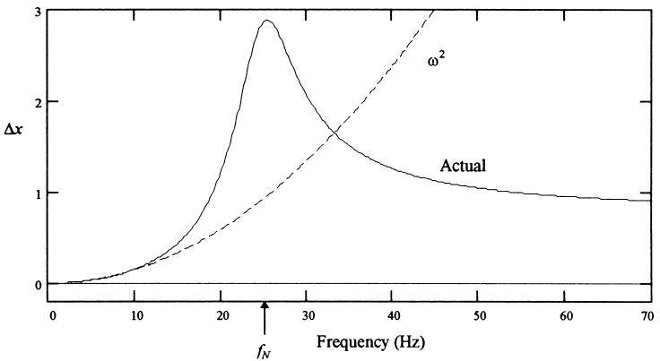
Accelerometer Under Vibration
Consider a spring–mass accelerometer mounted on a vibrating table.
Using \(ma = k\Delta x\) :
\[
\Delta x = -\frac{m x_0}{k}\, \omega^2 \sin(\omega t) \tag{29}
\]
Where:
\(x_0\) = table vibration amplitude\(\Delta x\) = relative mass motion\(\omega = 2\pi f\) = applied angular frequency
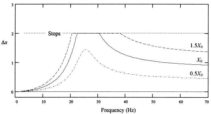
Key idea (ignoring resonance):
\(\Delta x \propto \omega^2 x_0\) → response grows with frequency squared.
Now tie in natural frequency: the simple prediction breaks down near \(f_N\) .
Use this to motivate choosing accelerometer specs based on the highest frequency of interest.
Spring‑mass system with the mass connected to the wiper of a potentiometer.
Mass motion → wiper motion → resistance change.
Requires excitation (voltage) + signal‑conditioning to get a usable voltage or current output.
Typical:
Natural frequency \(< 30\ \mathrm{Hz}\)
Used for steady‑state or low‑frequency acceleration.
Advantages: simple, low cost. Disadvantages: limited bandwidth, mechanical wear, not suited for harsh vibration.
Mention where such a sensor might appear today: low‑end tilt or level measurement, educational setups.
In many modern systems, potentiometers have been replaced by non‑contact methods (e.g., capacitive, optical) but the principle is still widely used.
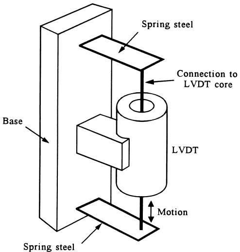
Use an LVDT (Linear Variable Differential Transformer) to measure mass displacement.
The LVDT core serves as the seismic mass.
Core motion → change in induced differential voltage → linear displacement signal.
Typical features:
Natural frequency \(\lesssim 80\ \mathrm{Hz}\)
Excellent linearity over range
Used for steady‑state and low‑frequency vibration measurements
Recall LVDT basics from earlier in the course: - AC excitation - Two secondary windings with differential output - Phase and magnitude encode direction and displacement
The accelerometer piggybacks on this concept by attaching the mass to the LVDT core.
Rely on changing magnetic flux and induced voltage.
Test mass is a permanent magnet .
As the magnet moves within a coil, it induces a voltage.
Key traits:
Output only when the mass is moving (no DC/static acceleration).
Used mainly for vibration and shock .
Natural frequency typically \(\lesssim 100\ \mathrm{Hz}\) .
Common application: geophones in oil exploration (measuring ground vibration).
These are dynamic‑only sensors: no output for constant acceleration (e.g., constant tilt).
Relate this to Faraday’s law and earlier inductive sensors.
Geophones are a nice example that crosses mechanical, geological, and ECE boundaries.
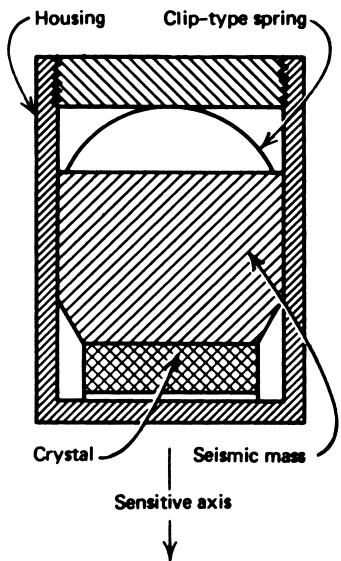
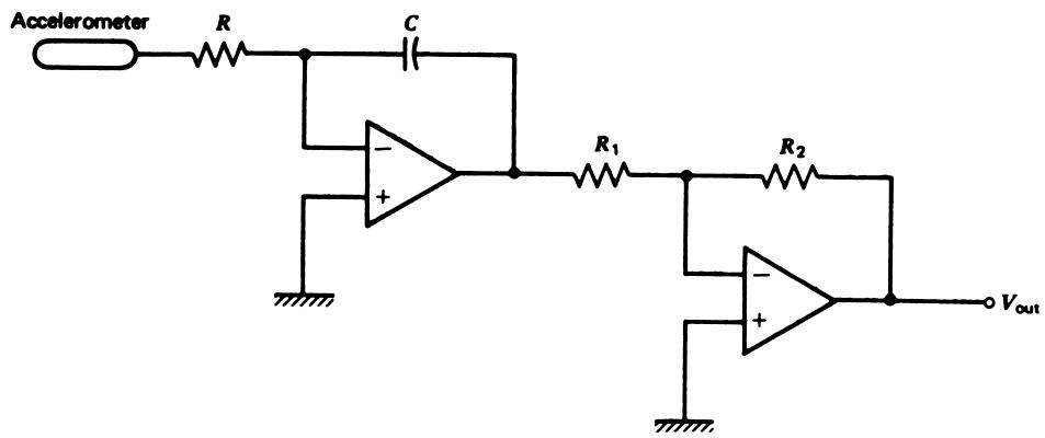
Use the piezoelectric effect : a crystal generates a voltage when mechanically stressed.
Test mass presses on a piezoelectric crystal.
Acceleration → inertial force \(F = ma\) on mass → stress on crystal → voltage.
Features:
Very high natural frequency (often \(> 5\ \mathrm{kHz}\) ).
Ideal for vibration and shock measurements.
Output: small voltage (mV range), very high source impedance → needs a high‑impedance, low‑noise amplifier .
Cannot truly measure DC acceleration (behaves like a high‑pass system).
Connect to crystal microphones, phonograph cartridges, and sonar transducers—same effect, different mechanical packaging.
Highlight that many commercial vibration sensors (for machinery monitoring) are piezoelectric accelerometers.
Pressure: Basic Concepts
Pressure = force per unit area exerted by a fluid (liquid or gas).
SI unit:
\(1\ \mathrm{Pa} = 1\ \mathrm{N/m^2}\)
Often use prefixes:
\(1\ \mathrm{kPa} = 10^3\ \mathrm{Pa}\) \(1\ \mathrm{MPa} = 10^6\ \mathrm{Pa}\)
Other common units:
\(\mathrm{psi}\) (pounds per square inch)
\(1\ \mathrm{psi} \approx 6.895\ \mathrm{kPa}\) torr (vacuum systems, low pressure)
\(1\ \mathrm{torr} \approx 133.3\ \mathrm{Pa}\)
atmosphere (atm): \(101.325\ \mathrm{kPa} \approx 14.7\ \mathrm{psi}\)
bar: \(1\ \mathrm{bar} = 100\ \mathrm{kPa}\)
Remind students: in design work, always keep track of units carefully; mixing psi, Pa, and “inches of water” is a common source of confusion.
Static vs Dynamic Pressure
Static pressure : fluid not moving relative to its container.
Example: water at rest in a vertical tank.
Dynamic pressure : pressure in a moving fluid depends on flow conditions.
Example: water in a hose; pressure changes when you open/close the nozzle.
Measurement systems must clearly state whether they are reading:
Static pressure only, orSome combination of static + dynamic (e.g., Pitot tubes in airflow).
In many process industries, “pressure” gauges effectively read static pressure.
In aerodynamics, dynamic pressure is critical (air speed, lift).
Gauge Pressure
Atmospheric pressure at sea level: ~\(14.7\ \mathrm{psi}\) (1 atm).
Often, we care about pressure relative to atmosphere , not absolute.
Absolute pressure \(p_{\text{abs}}\) : measured from vacuum.Gauge pressure \(p_g\) : relative to ambient atmosphere.
Relationship:
\[
p_g = p_{\text{abs}} - p_{\text{at}} \tag{30}
\]
In English units, use psig for gauge pressure.
A sealed container at \(14.7\ \mathrm{psi}\) absolute, sitting at sea level, has \(p_g = 0\)
Make sure students understand the difference between psia and psig; misreading this can cause severe design errors (e.g., choosing a vessel that cannot handle external vacuum).
Head Pressure (Hydrostatic Pressure)
For a liquid column of depth \(h\) :
SI form:
\[
p = \rho g h \tag{31}
\]
Where:
\(p\) = pressure (Pa)\(\rho\) = mass density \((\mathrm{kg/m^3})\) \(g \approx 9.8\ \mathrm{m/s^2}\) \(h\) = depth (m)
English form using weight density \(\rho_w\) \((\mathrm{lb/ft^3})\) :
\[
p = \rho_w h \tag{32}
\]
Where \(p\) is in \(\mathrm{lb/ft^2}\) .
To get psi , divide by 144 (since \(1\ \mathrm{ft^2} = 144\ \mathrm{in^2}\) ).
“Feet (or meters) of water” is a pressure unit : it’s shorthand for the pressure produced by that water column height.
Link back to level measurement: level → pressure → electrical signal.
Also note that density changes with temperature and with fluid type (e.g., oils vs water), something process engineers must consider.
To express in psi, we can use \(\rho_w \approx 62.4\ \mathrm{lb/ft^3}\) .
Pressure in \(\mathrm{lb/ft^2}\) :
\[
p = \rho_w h = (62.4\ \mathrm{lb/ft^3})(7.0\ \mathrm{ft}) = 437\ \mathrm{lb/ft^2}
\]
Convert to psi:
\[
p = \frac{437}{144}\ \mathrm{psi} \approx 3\ \mathrm{psi}
\]
Show that 21 kPa ≈ 3 psi is a good sanity check using \(1\ \mathrm{psi} \approx 6.9\ \mathrm{kPa}\) .
This example also sets up Example 17 later (using pressure sensors to measure level).
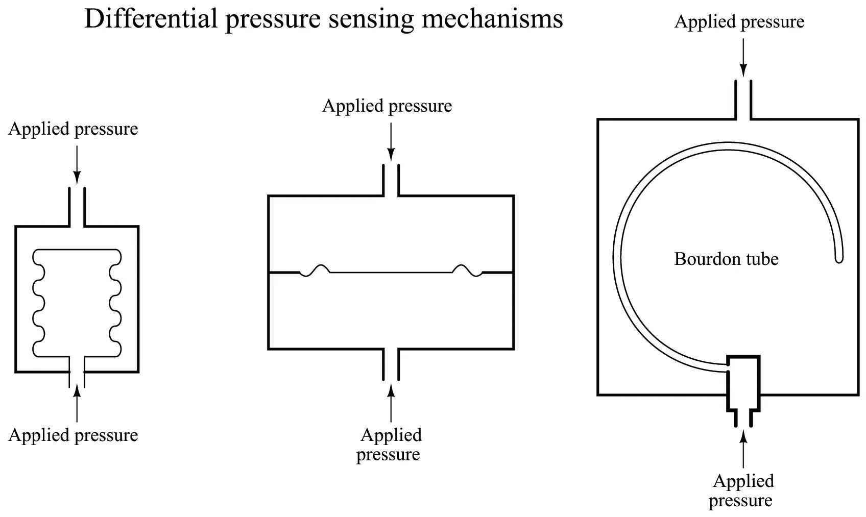
A thin flexible metal diaphragm with pressures \(p_1\) and \(p_2\) on each side.
Net force:
\[
F = (p_2 - p_1) A \tag{33}
\]
Where \(A\) is diaphragm area.
Diaphragm deflects until Hooke’s law force balances pressure force.
Deflection (displacement) is proportional to pressure difference .
Diaphragms form the heart of many pressure sensors, including modern MEMS devices.
In some designs, strain gauges are bonded directly to the diaphragm to measure strain (and thus pressure) without extra moving parts.
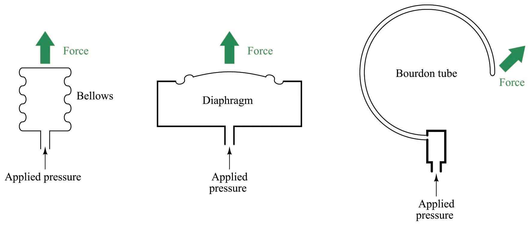
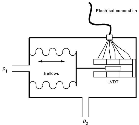
Bellows: an accordion‑like metal structure.
Pressure difference causes straight‑line expansion or contraction.
Displacement is nearly linear with \(\Delta p\) .
An LVDT measures bellows tip displacement.
Output voltage then becomes a linear function of pressure .
This is a classic example of chaining transducers:
pressure → mechanical element → LVDT → AC signal → demodulation → DC signal → controller.
Good place to review LVDT advantages: non‑contact, good linearity, robustness.
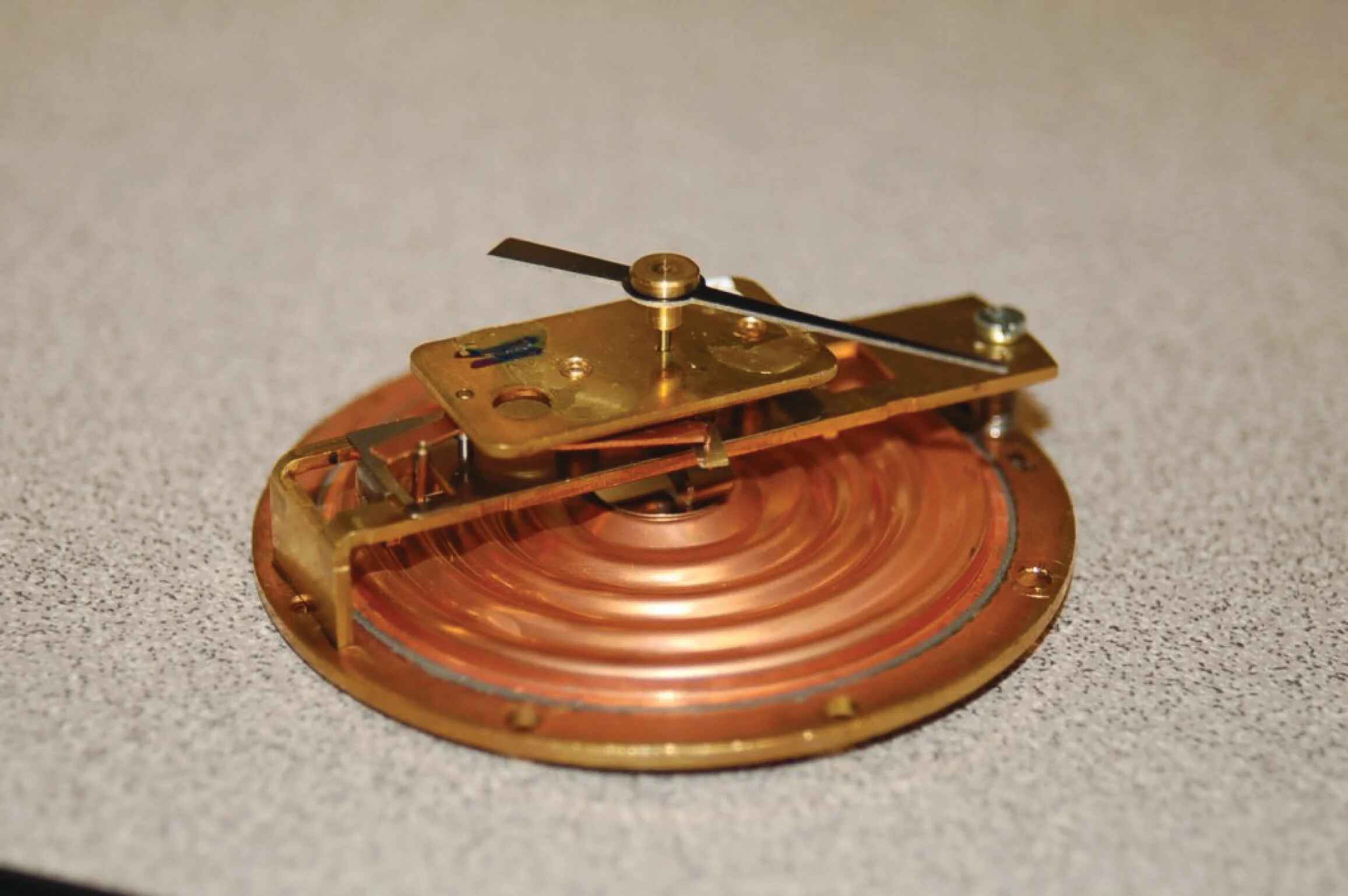
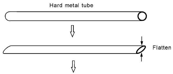
Operation:
If internal pressure > external pressure, tube tends to straighten .
If internal pressure < external, tube tends to curl more .
Tip motion is proportional to pressure difference.
Most analog round‑dial pressure gauges use a Bourdon tube driving a pointer via gears.
Explain how, for control applications, the tube tip motion is instead coupled to a displacement sensor (potentiometer, LVDT, etc.) to generate an electrical signal.
Mention mechanical hysteresis and long‑term drift as limitations for high‑precision work.
Electronic Pressure Conversion
Once we have displacement, we can convert to an electrical signal using:
Potentiometers – measure displacement as resistance.Strain gauges – often bonded directly to diaphragms.Inductive sensors – LVDTs, variable reluctance arrangements.Capacitive sensors – especially in MEMS devices.
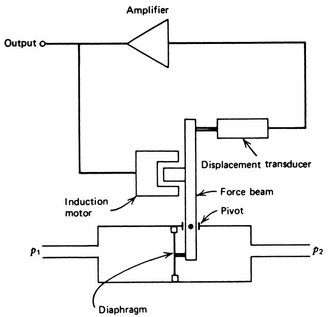
Advanced differential pressure cell with feedback:
A diaphragm senses \(\Delta p = p_1 - p_2\) .
A feedback actuator (e.g., induction motor) keeps diaphragm nearly centered.
Drive signal needed to null deflection becomes the pressure measurement .
This “force balance” or “null‑balance” architecture improves linearity, reduces mechanical wear, and allows accurate differential measurements over time.
It’s analogous to how some precision scales operate.
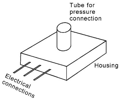
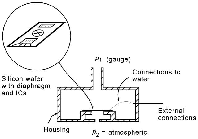
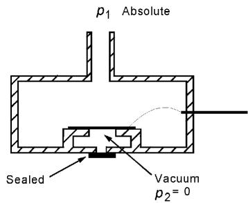
Integrated‑circuit technology enables compact solid‑state (SS) pressure sensors.
Inside:
A thin silicon diaphragm deflects under pressure.
Semiconductor strain gauges are diffused directly into the silicon.
On‑chip signal conditioning: amplification, temperature compensation, linearization.
Configurations:
Gauge : one side open to atmosphere.Absolute : one side sealed and evacuated.Differential : both sides connected to two different pressures.
These are the kind of sensors you find in automotive MAP (manifold absolute pressure) sensors, home appliances, medical devices, and industrial transmitters.
They often present a simple electrical interface: 5 V supply, ground, and analog output.
Sensor output:
\[
V = (25\ \mathrm{mV/kPa})(25.48\ \mathrm{kPa}) \approx 637\ \mathrm{mV} = 0.637\ \mathrm{V}
\]
So, for 0–2.0 m: 0–0.637 V.
Sensitivity per cm (200 cm range):
\[
S = \frac{637\ \mathrm{mV}}{200\ \mathrm{cm}} \approx 3.19\ \mathrm{mV/cm}
\]
Note how easily we go from pressure spec to level spec using \(p = \rho g h\) .
This is a typical instrumentation design task: selecting a pressure sensor for a desired level range and output voltage.
Summary / Key Points
Motion sensing starts from \(x(t)\) , \(v(t)\) , \(a(t)\) acceleration , which can be integrated to get velocity and position.
Types of motion: rectilinear, angular, vibration, and shock . Each calls for different sensor ranges and bandwidths.
The spring–mass accelerometer uses \(F = ma\) and \(F = k\Delta x\) ⇒ \(a = (k/m)\Delta x\) .
Natural frequency and damping determine how an accelerometer responds to vibration.
Avoid using near resonance (\(f \approx f_N\) ).
Accelerometer types:
Potentiometric and LVDT: good for steady or low‑frequency motion.
Variable‑reluctance: dynamic (vibration/shock) only.
Piezoelectric: high‑frequency vibration and shock; no DC.
Pressure is force per unit area , usually measured in Pa, psi, or related units.
Gauge pressure: \(p_g = p_{\text{abs}} - p_{\text{at}}\) .
Hydrostatic head: \(p = \rho g h\) .
Common pressure elements: diaphragm, bellows, Bourdon tube .
Displacement → potentiometer, LVDT, strain gauge, etc.
Solid‑state pressure sensors use silicon diaphragms with on‑chip strain gauges and conditioning, offering simple voltage outputs for 0–100 kPa ranges.
Encourage students to see the “big picture”: many very different‑looking instruments are based on the same mechanical and electrical principles.
Next steps: in labs or projects, they will calibrate real sensors, design conditioning circuits, and validate these equations with data.
Position from velocity (integral): \[x(t) = x(0) + \int_0^t v(\tau)\, d\tau \tag{19}\]
Sinusoidal vibration: \[x(t) = x_0 \sin(\omega t) \tag{20}\]
Angular frequency–frequency relation: \[\omega = 2\pi f \tag{21}\]
Vibration velocity: \[v(t) = \omega x_0 \cos(\omega t) \tag{22}\]
Vibration acceleration: \[a(t) = -\omega^2 x_0 \sin(\omega t) \tag{23}\]
Peak acceleration: \[a_{\text{peak}} = \omega^2 x_0 \tag{24}\]
Pressure & Head
Gauge pressure: \[p_g = p_{\text{abs}} - p_{\text{at}} \tag{30}\]
Hydrostatic pressure (SI): \[p = \rho g h \tag{31}\]
Hydrostatic pressure (English, weight density): \[p = \rho_w h \tag{32}\]
Diaphragm force: \[F = (p_2 - p_1)A \tag{33}\]
This slide is a good reference for exams and homework.
Encourage students to annotate with units and typical value scales (e.g., \(g = 9.8\ \mathrm{m/s^2}\) , \(1\ \mathrm{atm} = 101.3\ \mathrm{kPa}\) ).
Motion & Pressure Sensors – Interactive Deck
Warm‑Up: Unit Conversion (Acceleration)
Use Pyodide to convert acceleration from ft/s² to m/s² and g .
Prompt students:
What happens if you double the acceleration in ft/s²?
How does that reflect in g’s?
Explore Vibration: \(x(t)\) , \(v(t)\) , \(a(t)\)
Visualize sinusoidal vibration position, velocity, and acceleration.
Ask:
How does increasing \(f\) change \(a(t)\) ?
What happens if you reduce \(x_0\) by a factor of 10?
Reactive Vibration Explorer
Use sliders to control frequency and peak displacement , then see the vibration responses.
= Inputs. range ([1 , 50 ], {step : 1 , value : 10 , label : "Frequency f [Hz]" })= Inputs. range ([0.001 , 0.02 ], {step : 0.001 , value : 0.005 , label : "Peak displacement x₀ [m]" })
Notice how small changes in \(f\) have a big effect on peak acceleration because \(a_{\text{peak}} = \omega^2 x_0\) .
Have students:
Fix \(x_0\) and vary \(f\) ; observe peak \(a(t)\) .
Fix \(f\) and vary \(x_0\) ; compare sensitivity vs frequency.
Peak Acceleration vs Frequency
Plot \(a_{\text{peak}} = \omega^2 x_0\) \(x_0\) .
= Inputs. range ([5 , 100 ], {step : 5 , value : 50 , label : "Max frequency [Hz]" })= Inputs. select (new Map (["x₀ = 0.002 m" , 0.002 ], "x₀ = 0.005 m" , 0.005 ], "x₀ = 0.010 m" , 0.010 ], label : "Choose peak displacement" , value : 0.005 }
Ask students:
Doubling \(f_{\max}\) does what to the largest \(a_{\text{peak}}\) ?
How much does \(a_{\text{peak}}\) change when you switch from 0.002 m to 0.010 m?
Spring–Mass Accelerometer: Natural Frequency
Experiment with \(m\) , \(k\) and see how natural frequency changes.
Prompt:
What happens if you double the mass?
What if you double the spring constant?
Reactive Spring–Mass Designer
Adjust \(m\) and \(k\) via sliders and see \(f_N\) plus a suggested usable bandwidth .
= Inputs. range ([0.01 , 0.2 ], {step : 0.01 , value : 0.05 , label : "Seismic mass m [kg]" })= Inputs. range ([500 , 8000 ], {step : 500 , value : 3000 , label : "Spring constant k [N/m]" })
As a rule of thumb, use an accelerometer up to roughly \(f_N / 2.5\)
Ask:
For your current \(m\) and \(k\) , what is \(f_N\) ?
Is this accelerometer suitable for measuring 100 Hz vibration? Why or why not?
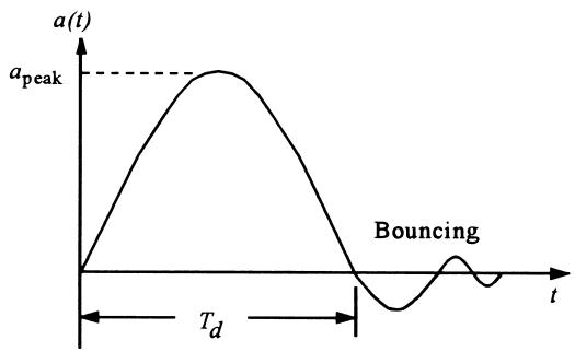
Shock Example: Drop Test Simulator
Simulate average deceleration from a drop of height \(h\) with shock duration \(T_d\) .
Invite:
Increase \(T_d_s\) to 0.02 s – what happens to average g’s?
Intuitively, why does a “softer landing” reduce shock?
Reactive Shock Explorer
Use sliders for drop height and shock duration ; plot average g as a function of \(h\) .
= Inputs. range ([0.5 , 5 ], {step : 0.5 , value : 2.0 , label : "Max drop height [m]" })= Inputs. range ([0.002 , 0.05 ], {step : 0.002 , value : 0.005 , label : "Shock duration T_d [s]" })
Discuss:
For a given product (e.g., phone), what combination of height and \(T_d\) is survivable given sensor and structure ratings?
Pressure: Unit Conversion Playground
Practice converting between Pa, kPa, psi, and atm.
Hydrostatic Pressure vs Depth
Use sliders to explore \(p = \rho g h\) for different depths and fluid densities.
= Inputs. range ([500 , 2000 ], {step : 50 , value : 1000 , label : "Density ρ [kg/m³]" })= Inputs. range ([0 , 5 ], {step : 0.1 , value : 2.0 , label : "Depth h [m]" })
Ask:
What is the slope of \(p\) vs \(h\) ? Does it match \(\rho g\) ?
How does changing \(\rho\) from 1000 to 1300 kg/m³ affect the curve?
Level‑to‑Voltage Mapping (SS Pressure Sensor)
Simulate Example 17: level measurement using a SS pressure sensor.
Encourage students to vary \(h_m\) and see linear scaling in \(V\) .
Ask how they would design an amplifier to convert this 0–0.637 V range to a standard 0–5 V signal.
Reactive Level Sensor Simulator
Interactively see how tank level maps to pressure and sensor output voltage.
= Inputs. range ([0 , 3 ], {step : 0.1 , value : 1.5 , label : "Liquid level h [m]" })= Inputs. range ([800 , 1500 ], {step : 50 , value : 1300 , label : "Density ρ [kg/m³]" })= Inputs. range ([10 , 50 ], {step : 5 , value : 25 , label : "Sensor sensitivity [mV/kPa]" })
Ask:
What output will you get at full tank (3 m)?
If you switch to a less dense fluid, how does that affect output for the same level?