Orientation of heavy steel plates in a rolling mill
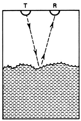
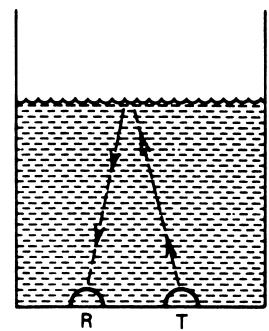
Liquid/solid level (a special kind of displacement)
Position of a workpiece in an automatic milling machine
Pressure → diaphragm deflection → displacement
We’ll look at three major electrical transduction mechanisms:
Resistive (potentiometric)
Capacitive / inductive
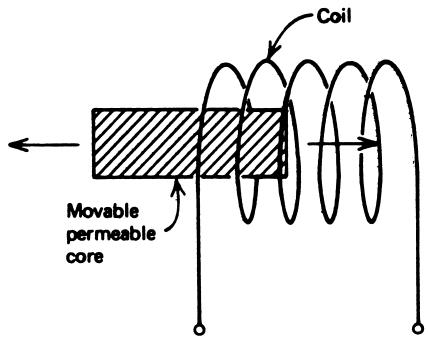
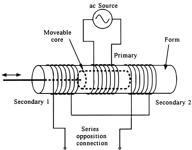
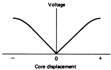
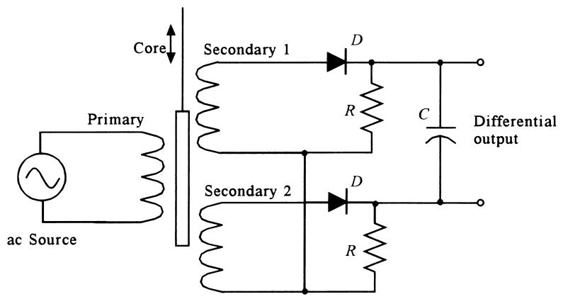
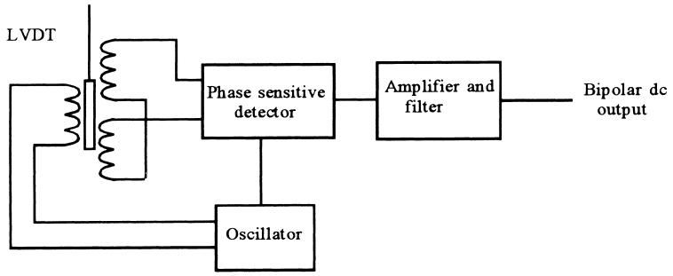
Variable‑reluctance (LVDT)
2.1 Potentiometric Displacement Sensors – Concept
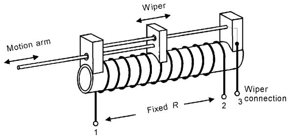
A potentiometric displacement sensor (potentiometer) uses a movable wiper on a resistor.
A resistive element with total resistance \(R\) between terminals 1 and 2
A wiper connected to an arm (mechanical linkage) at terminal 3
As the arm moves, the wiper slides along the resistor
The resistance between 3 and either end changes with position
Figure 1 Potentiometric displacement sensor.
Limitations:
Mechanical wear and friction of the wiper
Limited resolution in wire‑wound types (step size = spacing between turns)
Electrical noise from sliding contact
Potentiometer Resolution
In a wire‑wound potentiometer:
Distance between turns: \(\Delta x\)
Change in resistance between adjacent positions: \(\Delta R\)
The smallest resolvable displacement is roughly \(\Delta x\), assuming electronics can detect the resistance step \(\Delta R\).
More turns → smaller \(\Delta x\) → better resolution
But: more turns = higher resistance or longer device
Example 1 – Problem
Problem:
A potentiometric displacement sensor measures workpiece motion from 0 to \(10\ \mathrm{cm}\). The resistance changes linearly from 0 to \(1\ \mathrm{k}\Omega\) over this range.
Design signal conditioning that provides a linear 0–10 V output proportional to displacement.
Constraints:
Do not destroy the linearity between resistance and displacement.
Allowed tools: op‑amp circuits, DC references.
Example 1 – Why Not a Simple Divider?
If we put the variable resistor directly in a divider like this:
Vs --- R_fixed --- R_sensor --- GND
               |
             Vout
Then \[
V_\text{out} = V_s \frac{R_\text{sensor}}{R_\text{fixed} + R_\text{sensor}}
\]
This is nonlinear in \(R_\text{sensor}\) because of the denominator. So even if \(R_\text{sensor} \propto x\), you’ll get a nonlinear \(V_\text{out}(x)\).
We need a configuration where \(V_\text{out}\) is directly proportional to \(R_\text{sensor}\).
Example 1 – Solution Strategy (Op‑Amp)
Use the fact that for an inverting amplifier:
\[
V_\text{out} = -\frac{R_2}{R_1} V_\text{in}
\]
If we put the sensor as \(R_2\) (feedback resistor), then \(V_\text{out} \propto R_\text{sensor}\) (linearly).
We can:
Use a constant input voltage\(V_\text{in} =\) constant
Feed back through the variable resistance\(R_2 = R_\text{sensor}\)
Choose \(R_1\) to scale the output to 0–10 V over \(R_\text{sensor} = 0\)–\(1\ \mathrm{k}\Omega\)
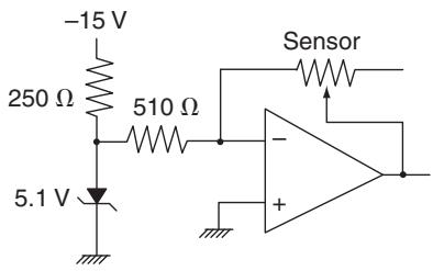
Example 1 – Detailed Solution
Use an inverting amplifier with:
\(R_2 = R_\text{sensor}\) (0 to \(1\ \text{k}\Omega\))
\(R_1\) fixed
\(V_\text{in} = -5.1\ \text{V}\) from a Zener diode reference
Then \[
V_\text{out} = -\frac{R_2}{R_1} V_\text{in}
\]
We want \(V_\text{out} = +10\ \text{V}\) at \(R_2 = 1000\ \Omega\):
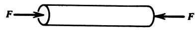
Often written as compressive stress, compressive strain
Figure 12b Compressional stress on a rod.
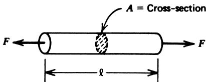
Stress units: \(\mathrm{N/m^2}\) (also called Pa, Pascal).
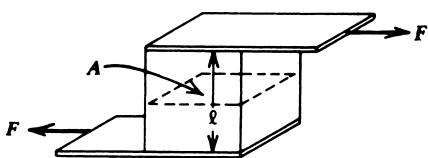
Shear Stress and Strain
Shear stress comes from a force couple that tries to slide one face relative to the other.
Stress:
\[
\tau = \frac{F}{A}
\]
Figure 13a Shear stress from a couple.
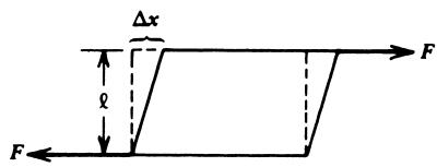
Shear strain is the lateral displacement normalized by thickness:
\[
\gamma = \frac{\Delta x}{l}
\]
Figure 13b Shear deformation.
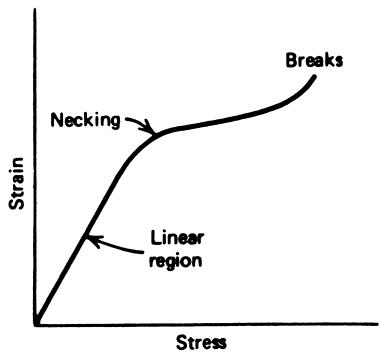
Stress–Strain Curves & Young’s Modulus
Figure 14 Typical stress–strain curve.
Key regions:
Linear (elastic) region: stress ∝ strain
Elastic limit: beyond which permanent deformation occurs
Necking → eventual fracture
In the linear region, we define:
\[
E = \frac{\text{stress}}{\text{strain}} = \frac{F/A}{\Delta l / l} \quad [\mathrm{N/m^2}]
\]
\(E\) is Young’s modulus (tensile/compressive).
Similarly for shear:
\[
M = \frac{\text{shear stress}}{\text{shear strain}} = \frac{F/A}{\Delta x/l}
\]
Modulus of Elasticity – Typical Values
Table 1: Young’s modulus \(E\)
Material
Modulus (\(\mathrm{N/m^2}\))
Aluminum
\(6.89 \times 10^{10}\)
Copper
\(11.73 \times 10^{10}\)
Steel
\(20.70 \times 10^{10}\)
Polyethylene plastic
\(3.45 \times 10^{8}\)
Soft materials (plastics) have much lower \(E\) → large strain for small stress.
Example – Strain in an Aluminum Beam
Problem:
Find the strain resulting from a tensile force of \(1000\ \mathrm{N}\) applied to a 10‑m aluminum beam with cross‑sectional area \(A = 4\times10^{-4}\ \mathrm{m^2}\).
Solution:
From table: \(E = 6.89\times10^{10}\ \mathrm{N/m^2}\).
Using
\[
E = \frac{F/A}{\Delta l / l} \Rightarrow \epsilon = \frac{\Delta l}{l} = \frac{F}{EA}
\]
Potentiometric sensors are simple but suffer from wear and limited resolution.
Capacitive and inductive sensors provide non‑contact measurements with better durability and sensitivity.
LVDTs are industry‑standard for linear displacement with excellent linearity and resolution.
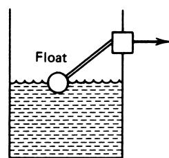
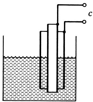
Level sensors
Many physical principles can be used: floats, capacitance, ultrasonics, and pressure.
Capacitive and ultrasonic methods allow non‑contact or non‑intrusive level measurement.
Strain and stress
Stress (force/area) and strain (relative deformation) are fundamental to many transducers.
Young’s modulus links stress and strain in the elastic region.
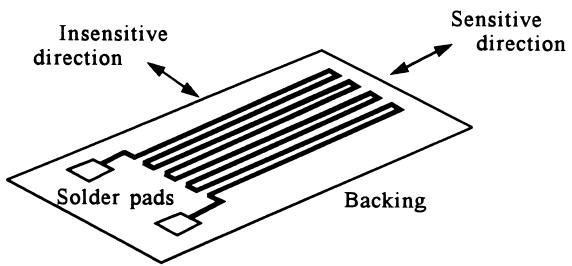
Strain gauges
Metal gauges use resistance change to measure strain; GF ≈ 2.
Semiconductor gauges offer much higher GF but are nonlinear and more temperature‑sensitive.
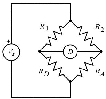
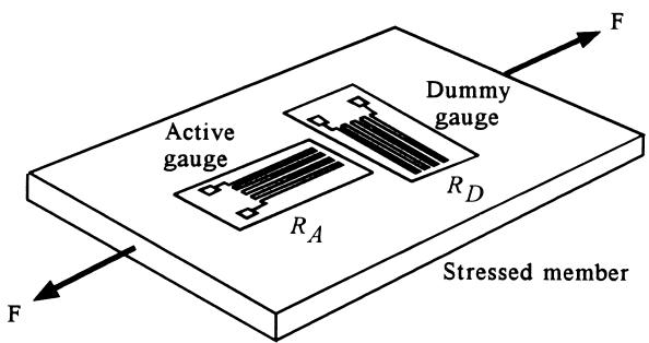
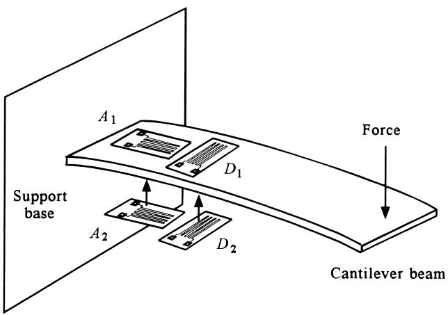
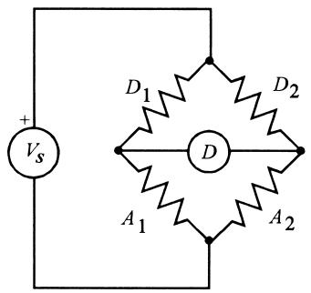
Wheatstone bridges with dummy gauges are crucial for sensitivity and temperature compensation.
Load cells
Use strain gauges on mechanical elements to convert force/weight into an electrical signal.
Output signals are typically in the microvolt to millivolt range and must be amplified.
Interactive Deck
1. Potentiometric Displacement Sensor – Direct Computation
Use this block to explore how a linear potentiometric sensor maps displacement → resistance → output voltage using the Example 1 circuit (inverting amplifier).