Data‑Acquisition Systems and Digital Data

Instruments 3.3

Imron Rosyadi

Learning Objectives

By the end of this session, you should be able to:

1. Describe the hardware blocks on a PC data-acquisition board (DAS) and their roles.
2. Explain how a PC communicates with a DAS through I/O ports and bus lines.
3. Trace the software flow to acquire a sample, including EOC polling and time-out handling.
4. Compute ADC resolution and relate digital codes to physical values (and vice versa).
5. Determine appropriate sampling rates and interpret aliasing and under‑sampling.
6. Explain and apply linearization techniques (equation‑based and table look‑up) for sensors.

Use this slide to set expectations and link to prior content:

• Previously: sensors, conditioning, basic ADC/DAC.
• Today: integrating all that into a PC/embedded system, plus thinking carefully about what we lose in digitizing (resolution, sampling, non-linearity).

Ask students: - “Who has used a USB DAQ, Arduino, or an oscilloscope with digital storage? That’s exactly the hardware-software chain we’ll formalize today.”

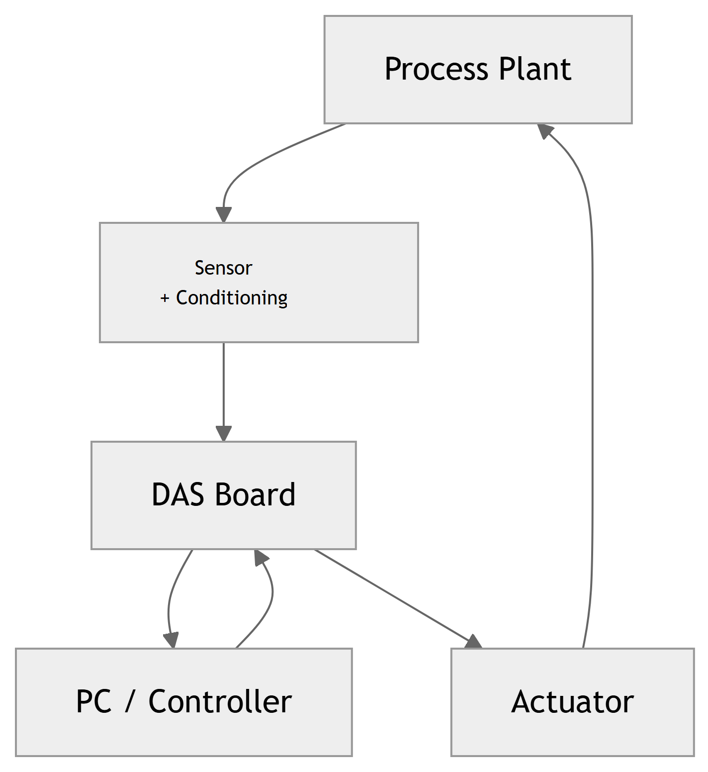
Big Picture: From Plant to PC

Control Loop Context

• Physical process (plant): temperature, pressure, flow, etc.
• Transducers + conditioning: produce an analog voltage or current.
• DAS (Data-Acquisition System):
  • Converts analog signals to digital for the PC.
  • Converts digital outputs from PC to analog actuators.
• PC / controller software: computes control action.

Note

The DAS is the bridge between the continuous analog world and the discrete digital world of the PC.

Emphasize that this is not just about desktop PCs: the same architecture appears in PLCs, microcontrollers, data loggers, and embedded systems.

Key idea: - Everything the controller knows about the process comes through this chain. Any limitations here (resolution, sampling, non-linearity) limit control performance, no matter how “smart” the algorithm is.

PC Architecture & Expansion Slots

• A typical PC uses a system bus with:
  • Address lines
  • Data lines
  • Control lines
• The CPU communicates with:
  • RAM, ROM, disks, etc.
  • Expansion slots for plug-in boards.
• DAS boards are PCBs that plug into expansion slots:
  • Use an industry-standard bus interface.
  • Appear as I/O ports or memory locations to the CPU.

Figure 29: Typical layout of a data-acquisition board for use in a personal computer expansion slot.

Point to Figure 29:

• Highlight the bus connector edge going into a PCI/ISA slot.
• Show students that the DAS is “just another peripheral” to the CPU, similar to a network card or graphics card.

Explain that from software’s point of view, DAS is visible through: - A set of I/O port addresses (e.g., 300H) or - Memory-mapped registers.

We will focus on the I/O port model here because that is what the example uses.

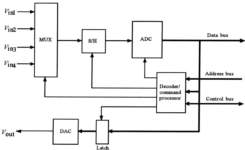
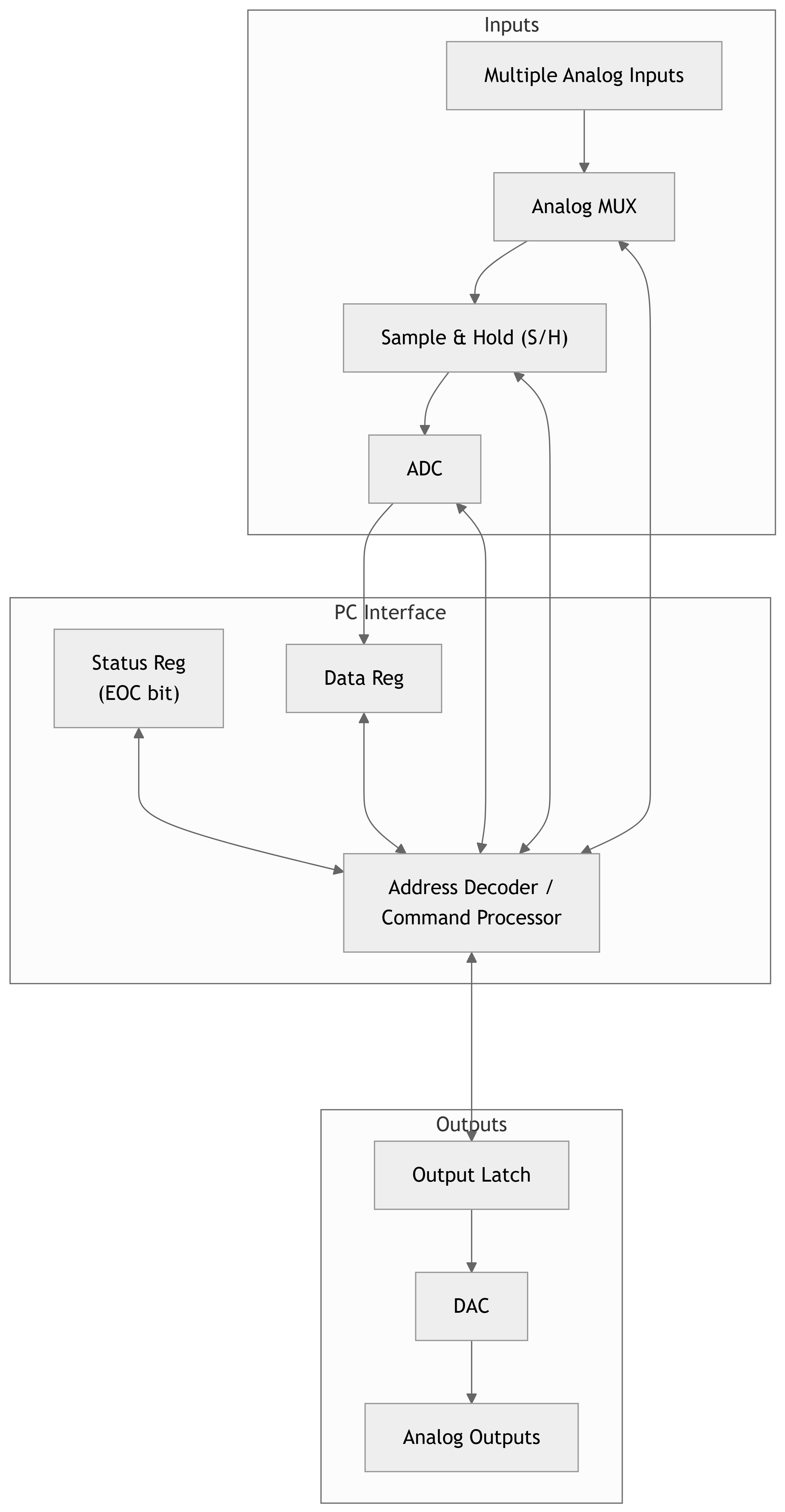
4.1 DAS Hardware – Block Diagram

Main Hardware Blocks

• Analog Inputs Side
  • Analog multiplexer (MUX)
  • Sample-and-hold (S/H)
  • ADC (successive approximation)
• Digital Interface
  • Address decoder / command processor
  • Status register (EOC, etc.)
  • Data register(s)
• Analog Outputs Side
  • Latch
  • DAC

Walk through the data path:

1. Many sensors → MUX → S/H → ADC → digital data register.
2. PC selects channel and starts conversion through the address decoder / command processor.
3. PC checks EOC via status register.
4. Digital outputs: PC writes a value → latch → DAC → analog output to actuator.

Reinforce that the S/H is essential when using a multi-channel MUX and a relatively slow ADC: it “freezes” the input long enough for conversion.

ADC & Sample-and-Hold (S/H)

• ADC (Analog-to-Digital Converter)
  • Typically successive-approximation type in DAS boards.
  • Key spec: conversion time (e.g., 25 µs).
• Sample-and-Hold (S/H)
  • Samples the input voltage and holds it constant while ADC converts.
  • Key spec: acquisition time (e.g., 10 µs to settle to within ½ LSB).

Total acquisition time per sample

\[ t_{\text{sample}} \approx t_{\text{acq}} + t_{\text{conv}} \]

Tip

To maximize throughput, you must account for both S/H acquisition time and ADC conversion time.

Clarify terminology:

• Acquisition time: time for S/H capacitor + circuitry to settle to within a specified error of the new input.
• Conversion time: time for the successive-approximation routine (or other ADC type) to produce a valid digital code.

If students have seen SAR ADC internals, relate that here; otherwise keep it intuitive: “the ADC needs a bit of time to ‘guess’ the code.”

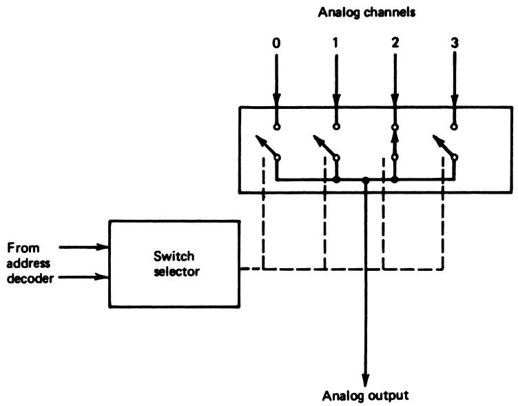
Analog Multiplexer (MUX)

• A DAS can select among multiple analog input channels.
• The analog MUX is like an electronic multi-position switch:
  • Only one input is connected to the S/H/ADC at a time.
  • Channels can often be scanned sequentially by software.
• Controlled by the address decoder / command processor on the board.

Figure 30: An analog multiplexer acts as a multiposition switch for selecting particular inputs to the ADC.

Use a simple analogy:

• Think of the MUX as a “rotary selector knob” driven by digital logic. The PC tells it, “Connect channel 3 now.”

Real-world application:

• Multichannel temperature monitoring: 8 thermocouples → 1 ADC via MUX to save cost and board space.

Mention that high-speed systems might use multiple ADCs in parallel to avoid the delay of sequential multiplexing.

Address Decoder / Command Processor

• The DAS is mapped to I/O port addresses (e.g., base port = 300H).
• The address decoder:
  • Watches the address bus and control lines.
  • Recognizes when the CPU is accessing its ports.
  • Routes read and write operations to:
    • Channel select register (for MUX).
    • Control register (to start conversion, initialize, etc.).
    • Status register (EOC bit, error bits).
    • DAC output latch.

Important

Software must use the correct base + offset addresses and bit patterns to control the DAS hardware.

Stress this is where “hardware meets software”:

• From the CPU point of view: “I just write a byte to 300H; magic happens.”
• On the board: that write is decoded, interpreted as “select channel 3 + start conversion,” etc.

Tie this to memory-mapped I/O vs. port-based I/O, but keep depth modest unless students already know OS/architecture details.

DAC and Output Latch

• Many DAS boards also provide analog outputs via DAC(s):
  • Used to control valves, motors, heaters, etc.
• Latch: holds the last value written by the CPU.
  • Prevents outputs from “glitching” during bus transactions.
• DAC: converts that latched digital value into a continuous analog output (unipolar or bipolar).

Example spec (from Example 25):

• 8-bit unipolar DAC
• 10.0‑V reference
• Output range: 0 V to just under 10 V (in 256 steps).

Remind students:

• DAC resolution, reference, and output type (unipolar/bipolar) determine what control signals we can generate.
• In many industrial systems, DAC output is then converted to 4–20 mA, 0–10 V field signals, etc.

You can quickly compute resolution: - For 8-bit DAC, 10 V range: - Step = 10 V / 256 ≈ 0.039 V per LSB.

4.2 DAS Software – Basic Flow

Figure 31: Software for data acquisition involves operations to start the ADC, test the EOC, and input the data.

Go through Figure 31 step by step, mapping each block to real instructions:

1. Select channel – write to channel selection register via I/O port.
2. Start conversion (SC) – write to control register.
3. Wait for EOC – typically polling a status bit in a loop.
4. Read data – read the data register when EOC is set.

Then highlight the problem: if EOC never comes (board failure, bus issue), the CPU can get stuck in the waiting loop. That motivates the need for a time-out.

DAS Software – Port & Status Details

• DAS is mapped to a base port address in hex: from 000H to FFFH; e.g., 300H.
• Often uses base + offset scheme:
  • BASE + 0 – data register.
  • BASE + 1 – control/status register (EOC bit, SC bit, etc.).
  • BASE + 2 – DAC register.

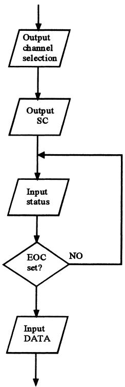
Typical software sequence to get one sample:

1. Write channel code to channel-select / control register.
2. Issue Start Convert (SC) command.
3. Repeatedly read status register until End Of Convert (EOC) bit signals done.
4. Read the data register to get the sample.

Warning

If the DAS fails and never sets EOC, a busy-wait loop can hang the entire system. Always include a time-out or use an interrupt.

Map this to the actual example that uses port 300H as base address.

Mention that in performance-critical systems, polling is inefficient; interrupts or DMA can free the CPU to do other work while the conversion runs.

But for many simple applications and labs, polling is fine and easier to understand.

Example 25 – Problem Setup

Given DAS specifications:

1. 8 input channels.
2. 8-bit bipolar ADC, 5.0-V reference, 25 µs conversion time.
3. S/H with 10 µs acquisition time.
4. 8-bit unipolar DAC with 10.0-V reference.

Task:

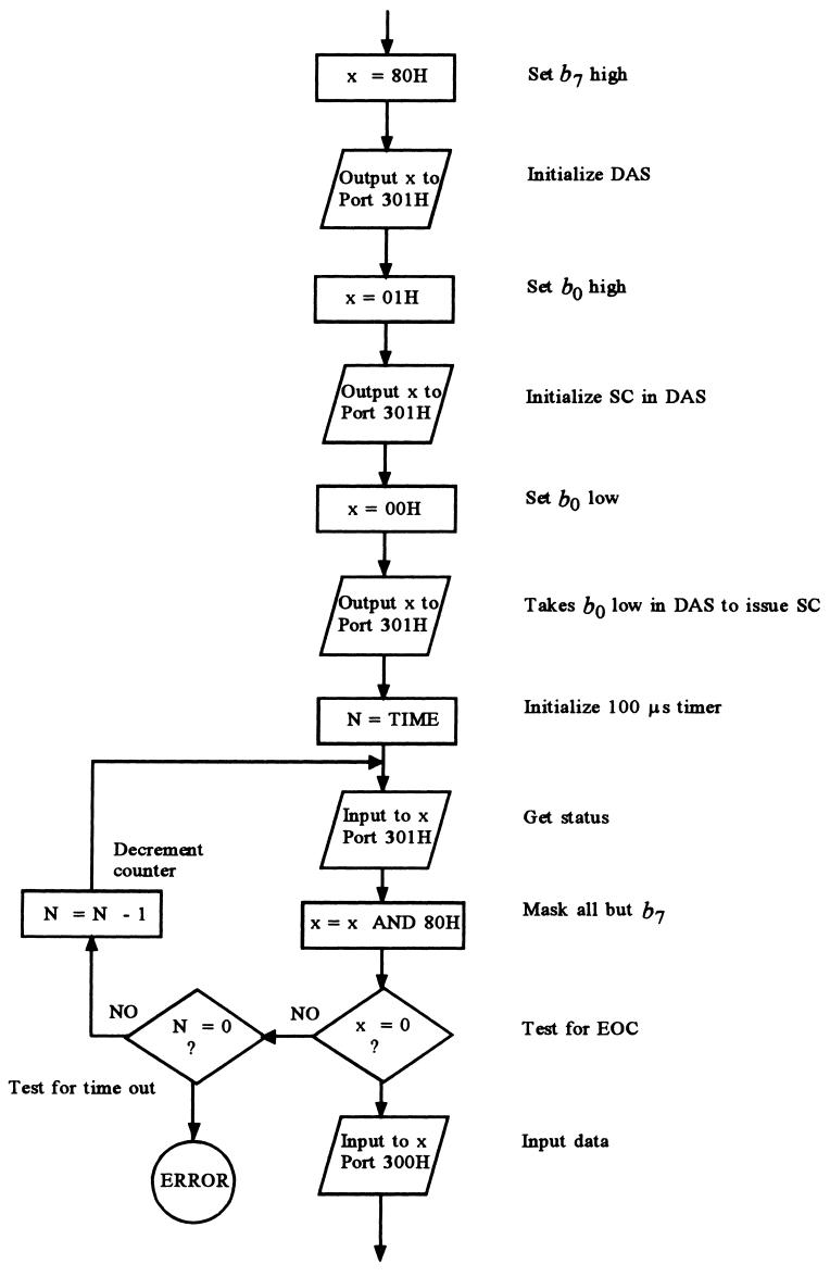
• Prepare a flowchart to take a sample from channel 3.
• Include a time-out that jumps to ERROR if EOC not issued after 100 µs.

Clarify:

• Channel 3 selection implies writing a byte where bit 3 = 1, bits others = 0 → 0000 1000b = 08H.
• Base port is 300H, so:
  • Channel select/data: 300H.
  • Status/control: 301H.
  • DAC: 302H.

The time-out must be implemented as a software loop whose total duration > 100 µs. Students will not compute the exact loop count here; they just represent it as a counter N.

Example 25 – Flowchart (Conceptual)

Address mapping (base is 000H to FFFH via switches; use BASE = 300H):

• BASE + 0
  • READ: inputs data sample from ADC.
  • WRITE: selects input channel (bit pattern).
    • \(b_0\) set → channel 0, …, \(b_7\) set → channel 7.
• BASE + 1
  • READ: inputs ADC status; EOC indicated by \(b_7\) going low.
  • WRITE:
    • If \(b_7\) high → initializes DAS.
    • When \(b_7\) low → taking \(b_0\) low issues SC.
• BASE + 2
  • READ: no action.
  • WRITE: sends data to DAC.

Figure 32: Solution to Example 25.

Talk through Figure 32:

1. Initialize: load port addresses (300H, 301H, 302H) into registers.
2. Select channel 3: write 08H to 300H.
3. Issue SC: write appropriate value to 301H to start conversion.
4. Wait for EOC:
   • Initialize counter N.
   • Loop: read 301H, check bit 7.
   • If EOC not set, decrement N.
   • If N = 0 before EOC, go to ERROR.
5. If EOC detected, read data from 300H.

Emphasize that the exact pattern written to 301H depends on the board’s control logic; the figure abstractly indicates what needs to happen.

This structure—poll with a counter for time-out—is very common in embedded firmware.

From Hardware to Information Loss

We now move from “how to get the data” to “what the digital data really means.”

Two key limitations:

1. Finite amplitude resolution
   • ADC outputs only one of \(2^n\) possible codes.
   • We lose knowledge of the exact analog value between codes.
2. Finite time resolution (sampling)
   • Controller only knows signal value at discrete sampling instants.
   • We are ignorant of behavior between samples.

Note

Even with a perfect controller algorithm, these two limitations can prevent meeting tight control specifications.

Transition slide: connect back to previous analog instrumentation coverage—where we often imagined continuous voltages being “known” exactly.

Here we quantify what we lose by digitizing, and how that affects control.

5.1 Digitized Value – ADC Mapping

The ADC output is an \(n\)‑bit binary representation of voltage \(V\) between \(V_{\min}\) and \(V_{\max}\).

Quantization relation:

\[ N = \frac{V - V_{\min}}{V_{\max} - V_{\min}} \, 2^n \tag{29} \]

• \(N\) = base-10 equivalent of output code (integer).
• Only the integer part is used.
• Assumes the ADC transitions from code \(2^n - 1\) to \(2^n\) exactly at \(V_{\max}\) (ideal behavior).

Resolution (LSB size) in volts:

\[ \Delta V = \frac{V_{\max} - V_{\min}}{2^n} \tag{30} \]

Tip

Resolution is the smallest change in input that produces a one-code change in output.

Emphasize:

• In practice, ADC outputs codes from 0 to \(2^n - 1\). The formula uses \(2^n\) to define code step size; the top code (all ones) corresponds to just below \(V_{\max}\).

Interpretation:

• After conversion, we only know \(V\) lies in an interval of width \(\Delta V\) around each code’s nominal value → this is the quantization uncertainty.

Example 26 – Setup

A temperature between \(100^\circ \mathrm{C}\) and \(300^\circ \mathrm{C}\) is converted to a 0–5.0 V signal. That signal feeds an 8‑bit ADC with a 5.0‑V reference.

Questions:

1. What is the actual measurement range of the system?

2. What is the resolution in °C?

3. What hex output results from \(169^\circ \mathrm{C}\)?

4. What temperature does a hex output of C5H represent?

Clarify analog chain:

• Sensor → conditioning → 0–5 V representing 100–300°C.
• ADC range: nominally 0–5 V → 8 bits.

The subtlety: the ADC saturates before 5.0 V, at (5 − 5/256) V, corresponding to ~299.22°C, so any higher temperature up to and beyond 300°C maps to FFH.

Thus, the actual representable range is slightly narrower than 100–300°C.

Example 26 – (a) Actual Measurement Range

ADC behavior at extremes:

• Top code FFH (255\(_{10}\)) occurs at \[ V = 5.0 \text{ V} - \frac{5.0}{256} = 4.98 \text{ V} \]
• That voltage corresponds to \[ T = 100^\circ \mathrm{C} + \frac{4.98}{5.0} (300^\circ \mathrm{C} - 100^\circ \mathrm{C}) = 299.22^\circ \mathrm{C} \]

So:

• FFH actually means any temperature ≥ 299.22°C (no code above FFH).
• At bottom: code 00H (0\(_{10}\)) is produced for all voltages less than \[ \frac{5.0}{256} = 0.0195 \text{ V} \]
• That corresponds to \[ T = 100^\circ \mathrm{C} + \frac{0.0195}{5.0} (300^\circ \mathrm{C} - 100^\circ \mathrm{C}) = 100.78^\circ \mathrm{C} \]

Therefore, actual measurement range: \[ 100.78^\circ \mathrm{C} \le T \le 299.22^\circ \mathrm{C} \]

Conceptual takeaway:

• The system was designed for 100–300°C, but the finite resolution of the ADC and its mapping to voltage means the extremes are not fully represented.
• At the top, the code “saturates,” merging everything ≥ 299.22°C into FFH.
• At the bottom, any temperature lower than 100.78°C is indistinguishable and gives 00H.

Example 26 – (b) Resolution

Temperature span:

\[ 300^\circ \mathrm{C} - 100^\circ \mathrm{C} = 200^\circ \mathrm{C} \]

ADC levels:

\[ 2^8 = 256 \]

Using Equation (30):

\[ \Delta T = \frac{200^\circ \mathrm{C}}{256} = 0.78^\circ \mathrm{C / bit} \]

Interpretation:

• If temperature is \(100^\circ \mathrm{C}\), output is 00H.
• It remains 00H until temperature reaches about \(100.78^\circ \mathrm{C}\), then jumps to 01H.
• For any reading, we are ignorant of the exact temperature within roughly ±0.39°C (half an LSB), often summarized as ±0.5 LSB.

Remind students:

• Quantization error is typically modeled as a uniform random variable in [−½ LSB, +½ LSB], assuming no other sources of error.

Connect to control requirement:

• If you need ±0.2°C control, but resolution is 0.78°C/bit, then you simply cannot meet that requirement with this measurement system.

Example 26 – (c) Code for 169°C

Use Equation (29):

\[ N = \frac{169 - 100}{300 - 100} 2^8 = \frac{69}{200} \times 256 \approx 88.32 \]

Take only integer part:

\[ N = 88_{10} \]

Convert 88\(_{10}\) to hex:

\[ 88_{10} = 58_{\text{H}} \]

So,

\[ 169^\circ \mathrm{C} \rightarrow \text{ADC output } 58\text{H} \]

Alternate method:

• Divide \((169 - 100)\) by resolution 0.78°C/bit: \[ \frac{69}{0.78} \approx 88.46 \Rightarrow 88_{10} \Rightarrow 58\text{H} \]

Difference between 88.32 and 88.46 is due to rounding in intermediate steps.

Highlight that any temperature between roughly 168.6°C and 169.4°C (about ±0.39°C) will map to the same code 58H.

This shows why digital temperature display may “jump” in discrete increments of ~0.8°C.

Example 26 – (d) Temperature for C5H

Given code C5H:

• C5H in decimal: \[ \text{C5H} = 12 \times 16 + 5 = 192 + 5 = 197_{10} \]

Use Equation (29) solved for \(T\):

Original: \[ N = \frac{T - 100}{300 - 100} 2^8 \]

Solve for \(T\):

\[ T = \frac{N}{2^8} (300 - 100) + 100 = \frac{197}{256} \times 200 + 100 \]

Compute:

\[ T = \frac{197 \times 200}{256} + 100 \approx 153.9 + 100 = 253.9^\circ \mathrm{C} \]

So,

\[ \text{C5H} \Rightarrow T \approx 253.9^\circ \mathrm{C} \]

Warning

Notice how much information loss there is: many distinct temperatures near 254°C all map to the same digital code C5H.

Reinforce:

• For a given ADC code, the true temperature lies in an interval of width ≈ 0.78°C.
• If the sensor and conditioning add more error, total measurement uncertainty is larger.

Ask: If we upgrade from 8-bit to 16-bit with same range, what is \(\Delta T\)?

• \(200^\circ \mathrm{C} / 65536 \approx 0.00305^\circ \mathrm{C}\)—now noise and other errors dominate.

Resolution vs. Noise Trade-off

With 16 bits and 5.0 V reference:

\[ \Delta V = \frac{5.0 \text{ V}}{65536} \approx 76.3 \,\mu\text{V} \]

• Extremely fine resolution.
• But in an industrial environment, noise from motors, switching, EMI, etc. is often much larger than tens of µV.

Important

Using more bits does not help once noise amplitude is larger than the LSB size. At that point, shielding, filtering, and grounding become critical.

Encourage students not to fix everything with “more bits.” There is a system-level trade-off:

• Too few bits → coarse resolution.
• Too many bits → not useful if the system is too noisy, and may even slow conversion or increase cost.

This sets up the next content on sampling in time.

5.2 Sampled Data Systems – Time Discretization

In addition to amplitude quantization, PC-based control systems also:

• Measure variables at discrete time instants only.
• Controller acts based on samples separated by \(t_s\) seconds.

Definitions:

• Sampling period: \(t_s\) (time between consecutive samples).
• Sampling frequency: \[ f_s = \frac{1}{t_s} \]

Two opposing constraints:

1. Maximum sampling rate
   • Limited by ADC conversion time + S/H acquisition + program execution time + communication delays.
2. Minimum sampling rate
   • Must be high enough to capture the signal dynamics and allow reconstruction/control.

Link back to hardware:

• A slow ADC and heavy software can limit how fast you can sample.
• Networked control (fieldbus, Ethernet) adds communication delays.

Then link to signal-processing view:

• Under-sampling → aliasing, missed disturbances, poor control.

Sampling Rate & Signal Reconstruction

Figure 33: The sampling rate can disguise actual signal details.

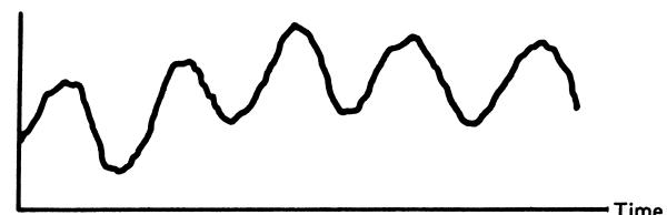
1. Actual analog signal

2. Too slow sampling: severe information loss

3. Aliasing: sampled data appears to have a false lower frequency

4. Adequate sampling: main features preserved

Explain each sub-figure qualitatively:

• 2. Sampling so slow that you miss most of the oscillations. Reconstructed signal (dashed) is a gross oversimplification.
• 3. Aliasing: the samples line up in such a way that you infer a slower oscillation than actually exists. This can completely mislead control design.
• 4. Faster sampling: the reconstructed signal approximates the original fairly well.

Connect to students’ experience: digital audio, video frame rate, oscilloscope sampling.

Practical Sampling Rule

Based on maximum signal frequency \(f_{\max}\):

\[ f_s \approx 10 f_{\max} \tag{31} \]

• That is, take about 10 samples per shortest signal period.
• Provides enough information for practical reconstruction and control.

Compare with Nyquist Theorem:

• Theoretically, a bandlimited signal with max frequency \(f_{\max}\) can be perfectly reconstructed if \[ f_s \ge 2 f_{\max} \]
• But:
  • Real industrial signals are not strictly bandlimited.
  • Perfect reconstruction at 2\(f_{\max}\) requires ideal conditions and often infinitely long reconstruction filters.

Note

Equation (31) is a practical engineering guideline, not a theorem. It gives a safety margin against aliasing and provides enough samples for control algorithms.

Resolve the apparent contradiction:

• Nyquist = minimum theoretical rate for perfect reconstruction of bandlimited signals.
• In practice: non-bandlimited, noise, system dynamics, and control design considerations → we choose a significantly higher sampling rate.

Ask students: “In audio, CD sampling is 44.1 kHz for ~20 kHz hearing range. That’s ~2.2 ×, not 10×—because continuous playback is the goal, not control of a physical process under uncertainty.”

Example 27 – Determining Sampling Period

Figure 34: Pressure data for Example 27.

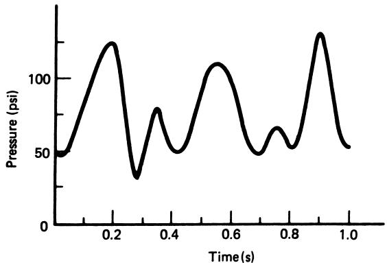
Problem:

• Pressure variations in a reaction vessel given as in Figure 34.
• Determine the maximum time between samples for a computer control system.

Solution outline:

1. Shortest time between any two peaks in data: \[ T_{\min} = 0.15 \text{ s} \]
2. Maximum signal frequency: \[ f_{\max} = \frac{1}{T_{\min}} = \frac{1}{0.15} \approx 6.7 \text{ Hz} \]
3. From Equation (31): \[ f_s = 10 f_{\max} \approx 67 \text{ Hz} \]
4. Max sampling interval: \[ t_s = \frac{1}{f_s} \approx 15 \text{ ms} \]

So, sampling no slower than every 15 ms.

Emphasize the idea of reading the maximum frequency from data:

• Look for the fastest oscillation (shortest peak-to-peak time), not the average.

This is typical when analyzing logged plant data to design a digital controller: we estimate the highest significant frequency and pick sampling accordingly.

Network & Fieldbus Delays – Example 28

Scenario:

• Control system uses a network (fieldbus) with heavy traffic.
• Bus limits cycle time to 450 ms to:
  • Request sample from sensor.
  • Receive sensor data at controller.
• Assume computer processing time negligible.

Question:

• What is the maximum controllable frequency of temperature variations in a reaction chamber?

Clarify “cycle time” here:

• There is delay for measurement request and response.
• We also need time to send control output back to final control element, often via the same bus.

So total time from “measure” to “actuate” is longer than the nominal bus cycle.

Example 28 – Solution

1. Measurement request + response: 450 ms.

2. Add output actuation delay (assumed 225 ms): \[ t_{\text{total}} = 0.45 \text{ s} + 0.225 \text{ s} = 0.675 \text{ s} \]

3. Effective sampling frequency: \[ f_s = \frac{1}{t_{\text{total}}} \approx \frac{1}{0.675} \approx 1.48 \text{ Hz} \]

4. From Equation (31): \[ f_{\max} = \frac{f_s}{10} \approx 0.148 \text{ Hz} \]

5. Corresponding period of maximum controllable variation: \[ T_{\min} = \frac{1}{f_{\max}} \approx 6.8 \text{ s} \]

So, the system can reasonably control temperature variations with periods ≥ 6.8 s. Faster variations will be under-sampled and poorly controlled.

Warning

Network delays effectively lower the sampling rate and limit how fast a process you can control. This is crucial in networked and distributed control systems.

Relate to real-world ECE:

• Fieldbus (PROFIBUS, Foundation Fieldbus), industrial Ethernet, wireless sensor networks.
• Heavy bus usage or congestion can degrade control performance, even if local controllers and ADCs are fast.

Good exam question: ask students to compute \(f_{\max}\) given bus cycle and processing time budgets.

5.3 Linearization – Why We Need It

Many sensors have nonlinear input-output relations.

Examples:

• Thermocouples: voltage vs. temperature is nonlinear.
• Some pressure sensors: \(V \propto \sqrt{p}\), etc.

After ADC, we get a digital value \(DV\) that reflects these nonlinearities:

• \(DV\) is often not directly proportional to the physical variable.
• Controller design and human interpretation are much easier if we have a digital value linearly related to the variable.

Two common software techniques:

1. Equation inversion (analytic linearization)
2. Table look-up (numeric linearization)

Position this as a pure software advantage of digital instrumentation:

• With analog-only systems, linearization would require complicated analog circuits.
• With digital systems, we can correct nonlinearities in software using any complexity we like.

Linearization by Equation – Concept

Suppose a transducer outputs voltage related to pressure \(p\) by

\[ V = K \sqrt{p} \tag{32} \]

The ADC converts \(V\) to a digital value \(DV\):

\[ DV \propto V \propto \sqrt{p} \tag{33} \]

We want a digital variable linearly related to \(p\).

Idea: square the measured quantity:

\[ DP = DV \times DV \propto p \tag{34} \]

Then, with appropriate scaling and offsets, \(DP\) can be made numerically equal to the actual pressure.

Tip

If the sensor relation is known and invertible, implement the inverse function in software to get a linearized variable.

Emphasize:

• Often the sensor manufacturer provides a calibration equation.
• In software, we can solve that equation for the physical variable in terms of \(DV\).

We will now see a concrete example where we explicitly invert the equation and include the ADC mapping.

Example 29 – Setup

Pressure \(p\) (50 to 400 psi) → measured by a transducer with output:

\[ V = 0.385 \sqrt{p} - 2.722 \]

This \(V\) feeds an ADC:

• Reference \(V_{\text{ref}} = 5.0\) V.
• Output codes 00H to FFH over the pressure range.

In software, DV = UDF(1) reads ADC result as decimal \(DV\) (0–255).

Goal: derive a linearization equation to compute \(p\) from \(DV\), such that \(p\) equals actual pressure (50–400 psi).

Key steps:

1. Express \(DV\) in terms of \(V\) using ADC scaling.
2. Substitute transducer relation for \(V\).
3. Solve resulting equation for \(p\) in terms of \(DV\).

Students should recognize that this is working backwards through the ADC and transducer.

Example 29 – Solution Steps

1. ADC relation:

   \[ DV = \frac{V}{V_{\text{ref}}} 2^8 = \frac{V}{5} \times 256 \]

   So \[ V = \frac{5}{256} DV \]

2. Sensor relation:

   \[ V = 0.385 \sqrt{p} - 2.722 \]

3. Substitute \(V\) from ADC into sensor equation:

   \[ 0.385 \sqrt{p} - 2.722 = \frac{5}{256} DV \]

4. Solve for \(\sqrt{p}\):

   \[ 0.385 \sqrt{p} = \frac{5}{256} DV + 2.722 \]

   \[ \sqrt{p} = \frac{\frac{5}{256} DV + 2.722}{0.385} \]

5. Solve for \(p\):

   \[ p = \left( \frac{5}{256 \cdot 0.385} DV + \frac{2.722}{0.385} \right)^2 \]

   Numerically simplifying coefficients gives:

   \[ p = (0.00507 \, DV + 7.071)^2 \]

So in code, after reading DV, we compute:

p = (0.00507 * DV + 7.071)^2

and p equals actual pressure in psi (50–400 psi).

Emphasize the pattern:

• Use algebra and calibration information to convert from “raw ADC counts” to “engineering units.”
• Often, this can be combined with other scaling factors in the code (e.g., to convert psi to bar).

In lab, you could have students acquire raw ADC counts and then apply a similar calibration formula.

Linearization by Table Look-up – Concept

Sometimes:

• No simple closed-form equation relates \(DV\) to the physical variable.
• Or equation is too complex / expensive to evaluate in embedded code.

Instead, use a table of calibration points:

• Memory holds a sequence of input codes and corresponding physical values.
• After each measurement:
  1. Search table for the nearest code(s) to the measured \(DV\).
  2. Use the corresponding physical value, possibly with interpolation between entries.

Analogy:

• Human uses thermocouple table: measure voltage, look up temperature row in table, maybe interpolate.

Note

Table look-up trades memory space for computational simplicity.

Mention embedded constraints:

• On small microcontrollers, multiplication and division can be relatively slow, whereas table look-up and addition, subtraction, etc. may be cheaper.

Also, sensors might provide only empirical calibration data, not neat formulas.

Table Look-up Flowchart

Figure 35: Linearization by table look-up can be accomplished by the operations in this flowchart.

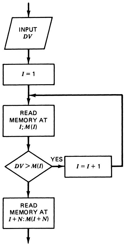
Assumed table structure:

• Inputs \(DV\) stored in ascending order in \(N\) memory locations.
• Corresponding physical values (e.g., temperature) stored in next \(N\) locations.

Lookup process:

1. Start at beginning of \(DV\) table.
2. Compare measured \(DV\) to table entries.
3. When a match or bracket is found:
   • If exact match: use corresponding physical value.
   • If bracketed between two entries: interpolate if desired.
4. Output the linearized value.

Explain indexing:

• Suppose DV table is at addresses TABLE to TABLE+N-1.
• Physical values are at TABLE+N to TABLE+2N-1.
• If input matches the \(I\)‑th DV entry, the physical value is found at address TABLE + N + I.

You can mention alternative searches (binary search for speed) and more elaborate interpolation (linear, spline) for high accuracy.

Problem & Solution Quick Practice

Problem 1 (Resolution):

A 12-bit ADC measures a 0–10 V signal.

1. What is the voltage resolution \(\Delta V\)?

2. If the measured code is 2048\(_{10}\), what is the nominal input voltage?

Solution:

\[ \Delta V = \frac{10 \text{ V}}{2^{12}} = \frac{10}{4096} \approx 2.44 \text{ mV} \]

2. For a code \(N\):

\[ V \approx N \cdot \Delta V = 2048 \times 2.44 \text{ mV} \approx 5.0 \text{ V} \]

Problem 2 (Sampling):

A process variable exhibits significant oscillations with period as small as 0.25 s.

What is the maximum sampling interval \(t_s\) you should use?

Solution:

• \(T_{\min} = 0.25\) s → \(f_{\max} = 1 / 0.25 = 4\) Hz.
• From Equation (31): \[ f_s = 10 f_{\max} = 40 \text{ Hz} \]
• Hence \[ t_s = 1 / f_s = 25 \text{ ms} \]

So choose \(t_s \le 25\) ms.

Use these quick problems as interactive checks:

• Ask students to compute answers individually or in pairs.
• Then reveal solution and discuss any pitfalls (bit count, where \(2^{12}=4096\) comes from, etc.).

Summary / Key Points

1. DAS hardware on a PC board typically includes:
   • Analog MUX, S/H, ADC, output latch, DAC, and address decoder / command processor.
2. PC–DAS communication uses bus lines and I/O port addresses (base + offset).
   • Software selects channels, starts conversions, checks EOC, and reads data.
3. Robust software must avoid infinite EOC-wait loops by using time-outs or interrupts.
4. Digital representation of analog values is limited by:
   • Resolution (quantization): \(\Delta V = (V_{\max} - V_{\min}) / 2^n\).
   • Sampling in time: sampling period \(t_s\) and frequency \(f_s=1/t_s\).
5. Practical sampling guideline:
   • Take about 10 samples per shortest signal period: \(f_s \approx 10 f_{\max}\).
6. Linearization compensates sensor + conditioning nonlinearities:
   • By equation inversion when analytic formulas exist.
   • By table lookup when relations are empirical or complex.

Invite questions that tie back to labs or projects:

• “In your Arduino/DAQ lab, where is the MUX? Where is the S/H? How do you start conversions?”
• “Have you seen aliasing on a digital oscilloscope—strange low-frequency patterns?”

Encourage them to think of each measurement system they encounter as an instantiation of these principles.

Formulas Summary

ADC mapping (ideal):

\[ N = \frac{V - V_{\min}}{V_{\max} - V_{\min}} \, 2^n \]

Resolution (quantization step):

\[ \Delta V = \frac{V_{\max} - V_{\min}}{2^n} \]

Sampling frequency and period:

\[ f_s = \frac{1}{t_s} \]

Practical sampling rule:

\[ f_s \approx 10 f_{\max} \]

Example linearization chain (from example 29):

ADC relation: \[ DV = \frac{V}{V_{\text{ref}}} 2^n \]

Transducer relation (example): \[ V = 0.385 \sqrt{p} - 2.722 \]

Combined & inverted: \[ p = (0.00507 \, DV + 7.071)^2 \]

Encourage students to memorize the structure of these formulas, not necessarily the numeric constants:

• Resolution scales as full-scale range divided by \(2^n\).
• Sampling frequency is the inverse of sample period.
• Linearization often means inverting a sensor’s calibration equation.

These will recur throughout digital instrumentation, signal processing, and control courses.

Interactive Deck

Interactive: ADC Resolution Calculator

Use this live code block to compute ADC resolution and explore how bit depth and voltage range affect it.

Tip

Try different values for bits and V_max. - What happens to ΔV when you double the number of bits? - What if you keep bits fixed but halve the voltage range?

Remind students: ΔV is given by Equation (30): \[ \Delta V = (V_{\max} - V_{\min}) / 2^n \] Have them confirm numerically that each additional bit halves the resolution step size.

Interactive: Code ↔︎ Voltage ↔︎ Temperature (Example 26)

We’ll model the temperature measurement system from Example 26:

• Temperature 100–300 °C → 0–5 V.
• 8-bit ADC with 5.0 V reference.

Use this interactive cell to convert between temperature, voltage, and ADC code.

Note

• Set T_input = 169.0 and confirm you get about 58H as in the text.
• Set code_input = 0xC5 and see that it maps to about 253.9 °C.

Point out that multiple temperatures map to the same code; students can see this by tweaking T_input slightly around 169 °C and confirming the integer code does not change until roughly ±0.39 °C (half an LSB).

Reactive: Visualizing Quantization (OJS + Pyodide + Plotly)

Use the sliders to choose bit depth and input voltage range. We’ll plot how the analog input is quantized by the ADC.

viewof bits = Inputs.range([2, 12], {step: 1, value: 8, label: "ADC bits (n)"})
viewof Vmax = Inputs.range([1, 10], {step: 0.5, value: 5, label: "V_max (volts)"})

Tip

Move the bits slider: - Watch the “staircase” get finer or coarser. - Notice how ΔV in the title changes as (1/2^n).

Explain that this is a mid-tread quantizer visualization: code intervals are roughly centered around each staircase level. Relate the shape of the staircase to the quantization error (vertical distance from gray line to blue line).

Interactive: Sampling Frequency & Nyquist vs. Practical Rule

Use this block to compare Nyquist rate and the practical 10× rule for a given maximum signal frequency.

Note

Try f_max = 6.7 Hz (as in Example 27) and compare the 15 ms practical period with the much larger Nyquist period (~75 ms).

Use this to reinforce why the control textbook recommends 10× as a “safe” rule: more samples per cycle give better tracking, robustness to noise, and tolerance for non-ideal signals.

Reactive: Sampling a Sine Wave – Aliasing Demo

Now you can see under-sampling and aliasing. Choose a signal frequency and sampling frequency.

viewof f_signal = Inputs.range([0.1, 10], {step: 0.1, value: 2.0, label: "Signal frequency f_signal (Hz)"})
viewof fs = Inputs.range([2, 50], {step: 1, value: 10, label: "Sampling frequency f_s (Hz)"})

Warning

• Try f_s just above 2 f_signal and then reduce f_s.
• Notice when the plotted samples mislead you about the real frequency (aliasing).

Ask students to locate conditions where f_s < 2 f_signal and they clearly see an aliased, slower apparent oscillation. Relate this visually to Figure 33(c) from the main deck.

Reactive: Sampling Rule of Thumb Visualization

Let’s visualize the 10× sampling guideline against Nyquist for a chosen ( f_{} ).

viewof fmax_slider = Inputs.range([0.5, 20], {step: 0.5, value: 5, label: "Max signal frequency f_max (Hz)"})

Note

This plot emphasizes that practical control often needs substantially more than the theoretical minimum sampling rate.

Encourage discussion: in what applications (e.g., audio recording) do we operate close to Nyquist, and in what applications (feedback control) do we prefer large oversampling factors?

Interactive: Simple Sensor Nonlinearity (Square-Root Pressure)

Play with a square-root sensor like the one used in the linearization examples:

\[ V = K \sqrt{p} \]

Tip

Try values for p_input and see that doubling pressure does not double the voltage. This nonlinearity must be corrected in software if we want a signal proportional to pressure.

Tie this back to the idea of equation-based linearization: software can square the ADC output (or apply a calibrated inverse equation) to obtain a value proportional to pressure.

Reactive: Linearization by Equation – From DV to p

We now implement a simplified version of Example 29 in a reactive way.

• You specify the raw ADC count DV.
• We compute the corresponding pressure p using the derived linearization formula.

viewof DV_input = Inputs.range([0, 255], {step: 1, value: 128, label: "ADC code DV (0–255)"})

Note

Drag the DV slider and watch how pressure changes nonlinearly with the raw ADC count.

Explain that although DV increments linearly, the mapping to p is quadratic here, undoing the original square-root relationship of the sensor. This demonstrates how software can “straighten” sensor nonlinearity.

Interactive: Table-Based Linearization Skeleton

Although we will not fully implement a table search here, you can experiment with a small lookup table by hand.

Tip

Change DV_meas and see which table entry it snaps to. More advanced implementations would interpolate between table points.

Connect this to Figure 35’s flowchart: our snippet corresponds to a very simple nearest-neighbor search; a more complete algorithm would include bounds checks and interpolation.

Wrap-Up: What Did You See?

Through these interactive blocks, you:

• Computed and visualized ADC resolution vs. bits and voltage range.
• Observed quantization as a staircase and associated uncertainty.
• Compared sampling frequencies under Nyquist vs. the practical 10× rule.
• Saw aliasing when sampling sinusoidal signals too slowly.
• Experimented with nonlinearity in sensor models and software-based linearization.
• Sketched table look-up behavior as an alternative linearization scheme.

Encourage students to copy and modify the code for their own experiments: - Try other sensor models (e.g., quadratic, exponential). - Add noise to the signals and see how it interacts with resolution and sampling. - Integrate this with microcontroller/DAQ experiments in the lab.