Units, Standards, and Definitions

Instrumentation 1.3

Imron Rosyadi

Learning Objectives

By the end of this session, you should be able to:

1. Explain the difference between static and dynamic (time) response of a sensor.
2. Describe and use the first‑order sensor time response and interpret the time constant τ.
3. Recognize second‑order (oscillatory) sensor responses and the roles of natural frequency and damping.
4. Apply concepts of significant figures to measurements, designs, and calculations.
5. Compute and interpret arithmetic mean and standard deviation for sensor data.
6. Relate standard deviation to sensor performance and the normal (bell) curve.

This entire deck covers two big themes:

1. Dynamic behavior of sensors (Section 7.x)
2. How we interpret measured values statistically (Section 8.x)

Keep tying this back to real process‑control loops:

• A “slow” sensor (large τ) can make a controller look bad even if the controller is fine.
• A “noisy” sensor (large σ) can make us mistrust individual readings.

7 Static vs Dynamic Behavior of a Sensor

Static transfer function

• Relationship between input and output when the input is constant in time.
• Example:
  • Thermocouple:
    • Input: temperature \(T\)
    • Output: voltage \(b\)
    • Static transfer: \(b = K T\) (for some range).
• Used to answer:
  • “What output should I get at 41 °C when everything has settled?”

Dynamic (time) response

• How the output changes with time when the input is changing in time.
• Independent of the static transfer function.
• Often characterized by how the sensor responds to a step input change.
• Used to answer:
  • “How long before the reading is close enough to the true value after a change?”

Note

The static transfer function tells you where the output will end up.
The dynamic (time) response tells you how fast and in what way it gets there.

Stress that an element can have:

• A perfectly linear static transfer function (great calibration),
• But terrible dynamic behavior (slow or oscillatory).

In control, both matter. Sensors are the “eyes” of the control loop—if the eyes are slow or shaky, the controller sees a distorted world.

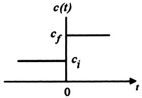
7 Step Response: How We Define Time Response

Figure 27: Sensor input step and delayed output response

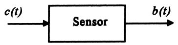
Concept:

• Input \(c(t)\) undergoes a step change at \(t = 0\):
  • From \(c_i\) (initial value) to \(c_f\) (final value).
• Static transfer function gives:
  • Before \(t=0\): output \(b_i\)
  • After settling: output \(b_f\)
• Real sensor:
  • Output \(b(t)\) lags and gradually transitions from \(b_i\) to \(b_f\).

Important

A step response is a standard way to characterize dynamic behavior: “If I change the input suddenly, how does the output react over time?”

Connect to ECE examples:

• Step input to a temperature sensor (placing it quickly into a hotter bath).
• Step change in pressure on a pressure transducer.
• LED photodiode suddenly illuminated.

Emphasize: we almost never have truly instantaneous changes in the real world, but the step response is a worst‑case test and is mathematically convenient.

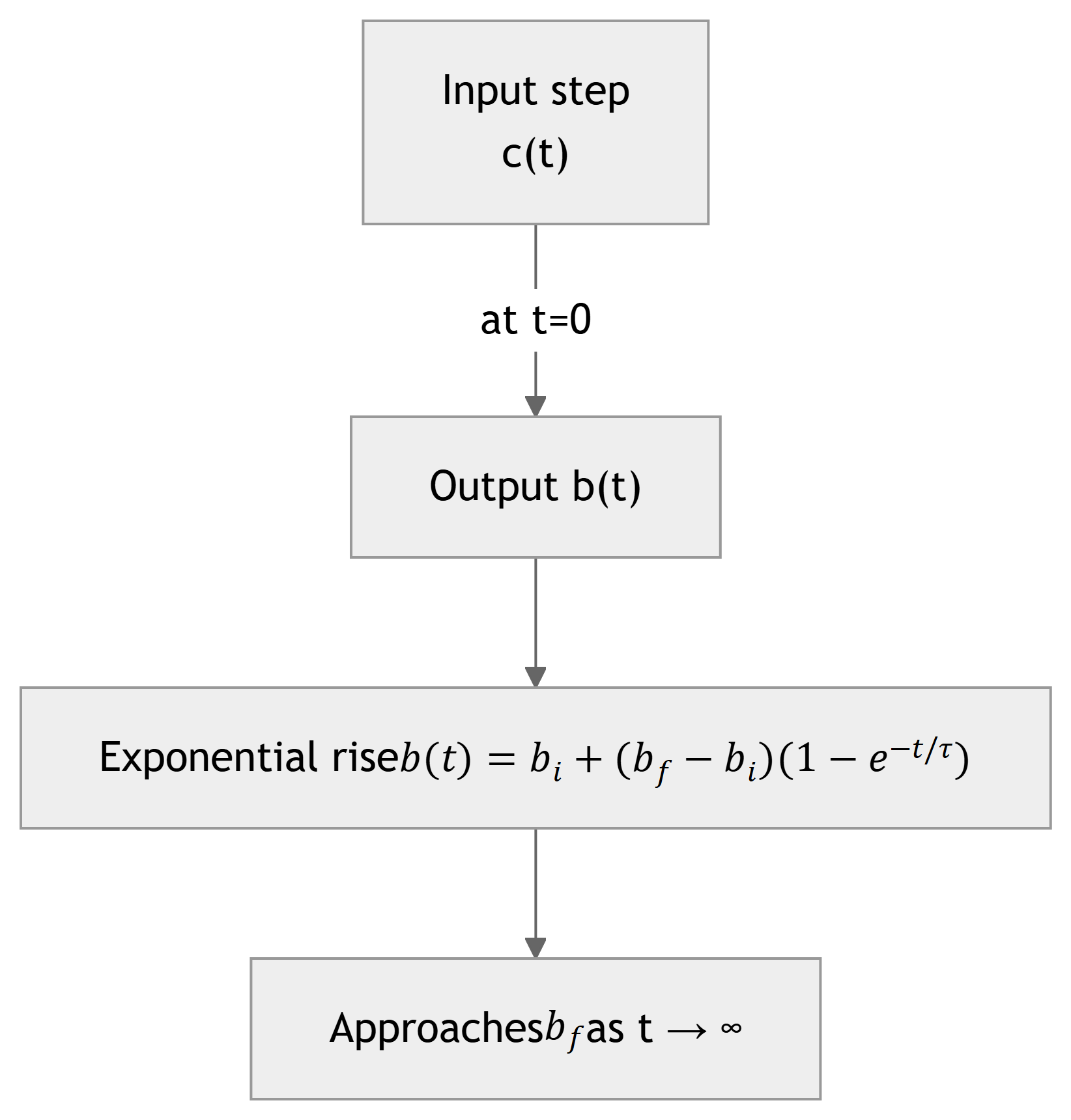
7.1 First‑Order Sensor Time Response

Figure 28: First-order exponential response to a step input

First‑order response characteristics:

• Smooth, exponential approach from \(b_i\) to \(b_f\).
• No oscillation or overshoot.
• Described by a first‑order differential equation.

General time response for \(t \ge 0\):

\[ b(t) = b_i + (b_f - b_i)\left[1 - e^{-t/\tau}\right] \tag{7} \]

• \(b_i\): initial output (before step).
• \(b_f\): final steady‑state output.
• \(\tau\): time constant of the sensor (units: seconds).

Mention that this form is identical to the response of:

• An RC circuit voltage to a step input (charging capacitor).
• A simple thermal system (lumped capacitance) heating up.

Students in ECE will recognize the similarity to filters. Encourage them to treat many sensors as “first‑order low‑pass elements” in the time domain.

7.1 Anatomy of the First‑Order Curve

Key properties of

\[ b(t) = b_i + (b_f - b_i)\left[1 - e^{-t/\tau}\right] \]

• At \(t = 0\):
  • \(b(0) = b_i\)
• As \(t \to \infty\):
  • \(b(t) \to b_f\)
• The bracket term is the fraction of total change achieved:

\[ \frac{b(t) - b_i}{b_f - b_i} = 1 - e^{-t/\tau} \tag{8} \]

Note

The dynamic model applies to the output \(b(t)\), not to the physical input \(c(t)\). The input is assumed to change instantly; the output cannot.

Point out subtle realism issue:

• Equation (7) predicts a finite initial slope at \(t=0\).
• Real physical sensors often start with zero slope due to internal physics. Despite that, (7) is an excellent approximation for most of the response and widely used in design and analysis.

7.1 Time Constant τ and the 63% Rule

Set \(t = \tau\) in Equation (8):

\[ b(\tau) - b_i = (b_f - b_i)\left[1 - e^{-1}\right] \tag{9} \]

Since \(e^{-1} \approx 0.3679\):

\[ b(\tau) - b_i \approx 0.632\, (b_f - b_i) \]

Interpretation:

• At \(t = \tau\), the output has reached about 63% of the total change.
• Common alternative names for \(\tau\):
  • 63% time
  • response time
  • e‑folding time

After 5τ, from (8):

\[ b(5\tau) - b_i \approx 0.993\, (b_f - b_i) \]

So after ≈ 5τ, the sensor output is extremely close to the final value (\(>99\%\) of the change).

Tip

Rule of thumb: for a first‑order sensor, - “1 τ to get ~63% there, - 3 τ to get ~95% there, - 5 τ to get essentially there.”

Connect to RC circuits:

• For a charging capacitor in an RC circuit, the same 63% rule applies.

Discuss practical design choices:

• If your process changes on a time scale of 0.1 s, but your sensor has τ = 2 s, the sensor is too slow and will significantly lag.

Interactive: Explore First‑Order Response

Adjust \(\tau\) and see how the response changes.

viewof tau = Inputs.range([0.1, 5], {step: 0.1, value: 1, label: "Time constant τ (s)"})
viewof t_max = Inputs.range([2, 20], {step: 1, value: 10, label: "Plot duration (s)"})

Ask students:

• When τ is small vs large, how does the curve look?
• How much time until the output is “good enough” (e.g., within 2% of final)?

Let them see that a larger τ means a much slower rise, illustrating why fast sensors (small τ) are valuable in many control applications.

Example 15: First‑Order Temperature Sensor

A sensor measures temperature linearly with static transfer function

• \(33 \text{ mV} / {}^\circ\text{C}\)
• Time constant: \(\tau = 1.5\) s

The process temperature changes instantly from

• \(20^\circ\text{C}\) to \(41^\circ\text{C}\) at \(t = 0\)

Tasks:

1. Find the sensor output at \(t = 0.75\) s.
2. Find the corresponding indicated temperature.
3. Compute the error in temperature relative to actual \(41^\circ\text{C}\).

Clarify:

• The input (temperature) itself is assumed to change instantly.
• The output (voltage) lags with first‑order response.

Students often mistakenly try to apply the exponential equation directly to the temperature input rather than the output variable.

Example 15: Step‑by‑Step Solution

1. Compute initial and final outputs from static transfer function:

\[ \begin{aligned} b_i &= (33 \text{ mV}/{}^\circ\text{C})(20^\circ\text{C}) = 660 \text{ mV} \\ b_f &= (33 \text{ mV}/{}^\circ\text{C})(41^\circ\text{C}) = 1353 \text{ mV} \end{aligned} \]

2. Apply first‑order time response at \(t = 0.75\) s:

\[ \begin{aligned} b(t) &= b_i + (b_f - b_i)\left[1 - e^{-t/\tau}\right] \\ b(0.75) &= 660 + (1353 - 660)\left[1 - e^{-0.75/1.5}\right] \\ &= 660 + 693\left[1 - e^{-0.5}\right] \\ &\approx 660 + 693\cdot(1 - 0.6065) \\ &\approx 932.7 \text{ mV} \end{aligned} \]

3. Convert output back to indicated temperature:

\[ T_\text{indicated} = \frac{b(t)}{33\text{ mV}/{}^\circ\text{C}} = \frac{932.7}{33} \approx 28.3^\circ\text{C} \]

4. Error relative to actual:

\[ \Delta T = T_\text{indicated} - T_\text{actual} = 28.3^\circ\text{C} - 41^\circ\text{C} = -12.7^\circ\text{C} \]

So, at 0.75 s, the sensor under‑reports by about 12.7 °C.

Warning

Time response analysis applies to the sensor output (voltage here), not to the actual process temperature.

Discuss “design implications”:

• If you used this sensor to control a heater with fast dynamics, the controller might continue to heat because it “thinks” the temperature is still low.
• Slow sensors can cause overshoot in control loops even if the plant is not inherently oscillatory.

Real‑Time Effects and Practical Guidance

• The ideal first‑order model assumes an instantaneous step in the input.
• Real processes often change more gradually → sensor lag is less severe.
• Our analysis is intentionally worst case.

Practical rule:

• A sensor can “track” variations well if the changes in the actual variable occur over times longer than about τ.

Tip

When choosing a sensor for a control loop:

• Compare sensor time constant τ with the time scale of process changes.
• For accurate tracking, aim for \(\tau_\text{sensor} \ll T_\text{process\_variation}\).

Give concrete ECE example:

• Monitoring CPU temperature: temperature changes relatively slowly, so a τ of several seconds is often fine.
• Monitoring RF signal envelope or high‑speed data: you need sensors with very small τ (e.g., fast ADCs, high‑bandwidth front‑ends).

7.2 Second‑Order Sensor Response

Some sensors show oscillatory behavior after a step input:

Figure 29: Oscillatory second-order response

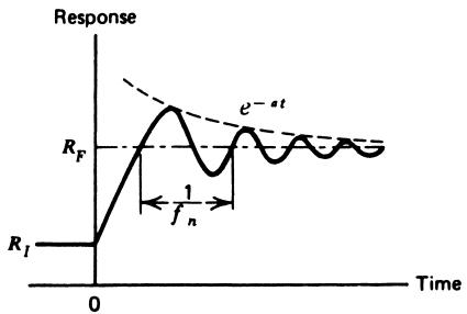
Characteristics:

• Output overshoots and undershoots around the final value.
• Oscillations decay over time due to damping.
• Described by a second‑order differential equation (similar to mass‑spring‑damper, RLC circuits).

7.2 Second‑Order Sensor Response

A generic damped oscillation can be written as:

\[ R(t) \propto R_0 e^{-a t} \sin(2\pi f_n t) \tag{10} \]

• \(R(t)\): sensor output component (oscillatory part).
• \(R_0\): amplitude.
• \(a\): damping constant (larger \(a\) → faster decay).
• \(f_n\): natural frequency (Hz) of oscillation.

Explain analogy:

• Think of a mechanical pressure sensor with internal mass and spring.
• A sudden pressure step can cause the mass to overshoot and oscillate.

In ECE, RLC circuits exhibit almost identical mathematics; students should link these concepts.

7.2 Second‑Order Response: Role of \(f_n\) and \(a\)

Natural frequency \(f_n\)

• Period of oscillation

\[ T_n = \frac{1}{f_n} \]

• Sensor can track inputs well if input variations are slower than this period.
• If the input changes faster than \(T_n\), the output can oscillate strongly.

Damping constant \(a\)

• Determines rate at which oscillations die out.
• Amplitude decays as \(e^{-a t}\).
• After time \(t = 1/a\):

\[ e^{-a(1/a)} = e^{-1} \approx 0.37 \]

→ amplitude dropped to about 37% of original.

Note

For second‑order sensors, two time‑related parameters matter:

• How fast they oscillate (\(f_n\)).
• How quickly oscillations die out (\(a\)).

Clarify that there is no simple universal step‑response formula like the first‑order case, because actual sensors can be:

• Underdamped (oscillatory)
• Critically damped
• Overdamped

The textbook’s Equation (10) is focusing on the underdamped oscillatory component, which is often the most problematic for measurement.

8 Significance and Statistics

Sensors and instruments don’t just lag; they also:

• Have inherent errors (bias, noise, etc.).
• Report values with limited precision (significant figures).
• Produce readings that vary randomly (random errors).

We need methods to:

1. Avoid claiming more precision than we really have (significant figures).
2. Summarize and interpret multiple readings (mean and standard deviation).

Transition: Up to now we’ve focused on dynamic error (time response). Now we focus on how we report and interpret numerical values from sensors.

Stress that this is essential in lab work, data sheets, and process control decisions.

8.1 Significant Figures: Why They Matter

Example: Digital meter reads 125 kΩ.

• This does not mean exactly \(125{,}000.000\ \Omega\).
• It means the resistance is closer to 125 kΩ than to 124 kΩ or 126 kΩ.

Definition: Significant figures are the digits that are actually known from a measurement or calculation.

• 125 kΩ → 3 significant figures.
• 2.21 mA → 3 significant figures.
• 5.0 V → 2 significant figures.

Important

Significant figures are about precision of the number you can justify, not about the correctness (accuracy) of that number.

Give mental model:

• Think of significant figures as “digits you are prepared to defend in a report.”
• Extra digits displayed on a calculator are often meaningless given the input data.

Significance in Measurement vs Accuracy

When using an instrument:

• Significance: number of readable digits or divisions.
• Accuracy: how close the reading is to the true value (given as ±% of reading or ±% of full scale).

They both matter, but are not the same.

Note

A 6‑digit meter with poor accuracy can give a very precise‑looking but wrong result. A 2‑digit meter with good accuracy can give a coarse but trustworthy result.

Example:

• A 4½ digit meter reading 12.34 V with ±5% accuracy.
• You should not claim “12.340 V exact”; your reading may be off by about 0.6 V.

Accuracy imposes an uncertainty range around the reading.

Example 16: Current Measurement and Uncertainty

A digital multimeter measures current through a 12.5 kΩ resistor as

• \(I = 2.21\text{ mA}\) on the 10 mA scale.
• Instrument accuracy: ±0.2% of full scale (FS).

Find:

1. Voltage across the resistor.
2. Uncertainty in the voltage.

Example 16: Solution

1. Determine significance and current uncertainty

• Reading: 2.21 mA → 3 significant figures.
• 10 mA scale, accuracy ±0.2% FS →

\[ \Delta I = 0.002 \times 10 \text{ mA} = 0.02 \text{ mA} \]

So \(I = 2.21 \pm 0.02\ \text{mA}\).

2. Compute nominal voltage using Ohm’s law:

\[ V = IR = (2.21\text{ mA})(12.5\text{ k}\Omega) = 27.625 \text{ V} \]

Given 3 significant figures in I, we report:

\[ V \approx 27.6\ \text{V} \]

3. Propagate uncertainty:

• Min current: 2.19 mA → \(V_\text{min} = 27.4\) V
• Max current: 2.23 mA → \(V_\text{max} = 27.9\) V

So uncertainty in V ≈ ±0.25 V, rounded to keep significance:

\[ V = 27.6 \pm 0.3\ \text{V} \]

Warning

Report both the nominal result and a reasonable uncertainty, keeping consistent significant figures.

Stress that the ±0.3 V uncertainty is rounded so that we do not imply more precision than is justified.

This is a typical format for reporting measurement results in labs.

Significance in Calculations

Rule: The result of a calculation can have no more significant figures than the least precise number used.

Example 17:

• Transfer function: \(22.4\ \text{mV}/{}^\circ\text{C}\) (3 sig figs).
• Measured voltage: \(412\ \text{mV}\) (3 sig figs).

Temperature:

\[ T = \frac{412\ \text{mV}}{22.4\ \text{mV}/{}^\circ\text{C}} = 18.392857^\circ\text{C} \]

But inputs have only 3 significant figures → answer must be:

\[ T = 18.4^\circ\text{C} \]

Note

Calculator output digits beyond the least significant input digit are not trustworthy and must be rounded off.

Encourage students to resist the temptation to keep all calculator digits in their final answer.

However, it is often useful to keep an extra guard digit in intermediate steps to reduce rounding error, then round at the end.

Design vs Measurement Significance

Design values (hypothetical, ideal):

• If a design specifies 1.1 kΩ, we treat it as exactly 1100 Ω.
• If we assign 4.7 V across it, then \(I = 4.7 / 1.1\text{k} = 4.2727272\ \text{mA}\) is okay as an exact calculation in design stage.

Measurement values (real, finite precision):

• If we measure \(R = 1.1\ \text{k}\Omega\) (2 sig figs) and \(V = 4.7\ \text{V}\) (2 sig figs),
  • Report \(I \approx 4.3\ \text{mA}\) (2 sig figs).

Important

In design problems: treat specified values as exact. In measurement problems: treat given digits as the significant figures.

Point out that textbooks often mix both kinds of problems; pay attention to context.

• If the problem says “design a circuit with 4.7 kΩ,” it’s a design value.
• If it says “a resistor was measured to be 4.7 kΩ,” it’s a measured value.

The treatment of significant figures is different in each case.

8.2 Statistics: Why Use Averages and Spread?

Consider many readings of the same variable:

• Each reading includes random errors.
• We want to estimate a “best value” and how spread out the readings are.

Two key tools:

1. Arithmetic mean (average)
2. Standard deviation (measure of spread)

Note

A single reading can be misleading. Collections of readings + statistics give a more reliable picture of the true value and sensor performance.

Connect to calibration:

• When calibrating a sensor, we often take multiple readings at each calibration point.
• The mean helps identify the sensor’s systematic behavior; the standard deviation indicates measurement repeatability.

Arithmetic Mean

Given \(n\) measurements \(x_1, x_2, \dots, x_n\):

\[ \bar{x} = \frac{x_1 + x_2 + \cdots + x_n}{n} \tag{11} \]

Using the summation symbol:

\[ \bar{x} = \frac{\sum x_i}{n} \tag{12} \]

• \(\bar{x}\): arithmetic mean
• \(\sum x_i\): sum of all values
• \(n\): number of values

Tip

The mean is often our best estimate of the “true” value when random errors are present and no other biases are known.

Remind students that for digital systems, averaging is easy and helps reduce random noise (e.g., oversampling and averaging ADC readings).

Also, mention that averaging multiple sensor readings in different locations (e.g., temperatures in a reactor) provides a meaningful overall process variable.

Standard Deviation: Measuring Spread

Given \(n\) values \(x_1, x_2, \ldots, x_n\) with mean \(\bar{x}\):

1. Compute deviations:

\[ d_i = x_i - \bar{x} \]

2. Standard deviation:

\[ \sigma = \sqrt{\frac{d_1^2 + d_2^2 + \cdots + d_n^2}{n - 1}} \tag{13} \]

Or, with summation:

\[ \sigma = \sqrt{\frac{\sum d_i^2}{n - 1}} \tag{14} \]

Interpretation:

• Larger \(\sigma\) → readings are more spread out around the mean.
• Smaller \(\sigma\) → readings cluster more tightly around the mean.

Note

In experimental practice, we use \(n-1\) in the denominator (not \(n\)) to get an unbiased estimate of the population variance.

Remind:

• \(n\) is the number of samples; using \(n-1\) is standard in experimental statistics (sample standard deviation).
• Students will see this again in probability and statistics courses.

Example 18: Room Temperature Measurements

Eight temperature readings in a room:

• \(21.2^\circ\), \(25.0^\circ\), \(18.5^\circ\), \(22.1^\circ\), \(19.7^\circ\), \(27.1^\circ\), \(19.0^\circ\), \(20.0^\circ\) C

Find:

1. Arithmetic mean temperature.
2. Standard deviation.

Example 18: Solution

1. Mean temperature using Equation (11):

\[ \bar{T} = \frac{21.2 + 25.0 + 18.5 + 22.1 + 19.7 + 27.1 + 19.0 + 20.0}{8} = 21.6^\circ\text{C} \]

2. Standard deviation using Equation (13):

\[ \sigma = \sqrt{\frac{(21.2 - 21.6)^2 + (25.0 - 21.6)^2 + \cdots + (20.0 - 21.6)^2}{8 - 1}} \]

Result:

\[ \sigma = 3.04^\circ\text{C} \]

Interpretation:

• Mean room temperature ≈ 21.6 °C.
• Typical variation about mean is about 3 °C across sampled locations.

Point out physical interpretation:

• Could indicate poor mixing of air or non‑uniform heating.
• In process control, such spatial variability may matter (e.g., in reactors, ovens).

Relate: a smaller σ would mean temperature is more uniform across the room.

Visualizing Standard Deviation

Figure 30: Distributions for two sensors with different σ

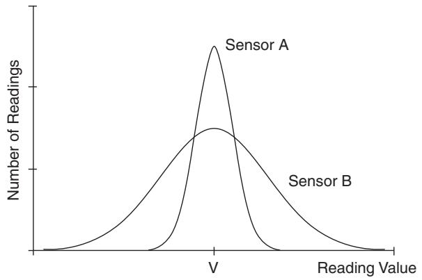
• Both sensors measure the same true value \(V\).
• Sensor A: narrow distribution → small σ.
• Sensor B: wide distribution → large σ.

Implications:

• Any single reading from Sensor A is more likely to be close to \(V\).
• For Sensor B, readings vary more; averaging more samples may be needed to estimate \(V\).

Important

Standard deviation quantifies repeatability and noise level of sensor readings.

Relate to ECE:

• Compare two ADCs: one with low input‑referred noise (low σ), and another noisier ADC (high σ).
• In digital communications, σ is related to noise power and error probability.

Normal (Gaussian) Distribution and σ

If we assume:

• Errors are truly random, and
• We have a large number of samples,

the distribution of readings often approaches a normal (bell) curve.

For a normal distribution:

1. About 68% of readings lie within ±1σ of the mean.
2. About 95.5% within ±2σ.
3. About 99.7% within ±3σ.

Example: Mean pressure 44 psi.

• Case 1: \(\sigma = 14\) psi → 68% of readings between 30 and 58 psi.
• Case 2: \(\sigma = 3\) psi → 68% of readings between 41 and 47 psi.

Note

Smaller σ → tighter cluster → more reliable individual readings.

Mention this rule as the 68‑95‑99.7 rule.

This helps students reason about the probability of extreme measurement values and how likely an outlier is.

Example 19: Evaluating a Control System with Statistics

A system packages potato chips into 200 g bags.

Samples (15 bags) drawn before control system installed:

201, 205, 197, 185, 202, 207, 215, 220, 179, 201, 197, 221, 202, 200, 195

Samples after control system installed:

197, 202, 193, 210, 207, 195, 199, 202, 193, 195, 201, 201, 200, 189, 197

Tasks:

• Compute mean and standard deviation before and after.
• Evaluate whether the system improved performance.

Example 19: Solution and Interpretation

Using Equations (12) and (14):

Before control system:

• Mean:

\[ \bar{W}_b = 202\ \text{g} \]

• Standard deviation:

\[ \sigma_b = 11\ \text{g} \]

After control system:

• Mean:

\[ \bar{W}_a = 199\ \text{g} \]

• Standard deviation:

\[ \sigma_a = 5\ \text{g} \]

Example 19: Solution and Interpretation

Interpretation:

• Target is 200 g.
• Mean moved from 202 g → 199 g → closer to target overall.
• Spread (σ) reduced by about a factor of 2 (11 g → 5 g).

If we use the ±3σ rule:

• Before: \(99\%\) of bags ≈ \(202 \pm 33\) g → 169 to 235 g.
• After: \(99\%\) of bags ≈ \(199 \pm 15\) g → 184 to 214 g.

So, the control system tightened the distribution and reduced systematic deviation from target.

Tip

Combining mean and standard deviation gives a richer view of system performance than either alone.

Note that even though the mean moved slightly below 200 g, the reduced spread is usually desirable (less giveaway, more consistency).

This example strongly parallels sensor calibration:

• After calibration or control redesign, we want outputs closer to target and less variable.

Summary / Key Points

1. Static vs dynamic response
   • Static transfer function: relates steady‑state output to input.
   • Dynamic (time) response: describes how output changes over time after input changes.
2. First‑order sensor response
   • Exponential approach: \(b(t) = b_i + (b_f - b_i)(1 - e^{-t/\tau})\).
   • Time constant τ:
     • 1τ → ~63% of final change.
     • 5τ → ~99% of final change.
3. Second‑order response
   • Oscillatory with damping: \(R(t) \propto R_0 e^{-a t} \sin(2\pi f_n t)\).
   • Natural frequency \(f_n\) and damping constant \(a\) are sensor characteristics.

Summary / Key Points

4. Significant figures
   • Never claim more digits than measurement supports.
   • Calculated results cannot have more significant figures than the least precise input.
   • Design values vs measurement values are treated differently.
5. Statistics of measurements
   • Mean \(\bar{x}\): central value of readings.
   • Standard deviation σ: spread of readings; quantifies repeatability/noise.
   • Normal distribution:
     • ~68% within ±1σ, ~95.5% within ±2σ, ~99.7% within ±3σ.

Encourage students to:

• Always check both dynamic characteristics and statistical behavior when evaluating a sensor for a control application.
• Use τ, σ, significant figures, and uncertainty consciously in lab reports and designs.

Formula Summary

First‑order sensor step response:

\[ b(t) = b_i + (b_f - b_i)\left[1 - e^{-t/\tau}\right] \tag{7} \]

Fraction of total change achieved at time \(t\):

\[ \frac{b(t) - b_i}{b_f - b_i} = 1 - e^{-t/\tau} \tag{8} \]

At \(t = \tau\):

\[ b(\tau) - b_i = (1 - e^{-1})(b_f - b_i) \approx 0.632 (b_f - b_i) \tag{9} \]

Second‑order oscillatory response component:

\[ R(t) \propto R_0 e^{-a t} \sin(2\pi f_n t) \tag{10} \]

Formula Summary

Arithmetic mean:

\[ \bar{x} = \frac{x_1 + x_2 + \cdots + x_n}{n} \tag{11} \]

or

\[ \bar{x} = \frac{\sum x_i}{n} \tag{12} \]

Standard deviation (sample):

\[ \sigma = \sqrt{\frac{d_1^2 + d_2^2 + \cdots + d_n^2}{n - 1}} \quad\text{where}\quad d_i = x_i - \bar{x} \tag{13} \]

or

\[ \sigma = \sqrt{\frac{\sum d_i^2}{n - 1}} \tag{14} \]

Encourage students to memorize or have handy:

• First‑order response equation and 1τ ≈ 63% rule.
• Mean and standard deviation formulas.

Everything else (e.g., significance rules, normal distribution properties) is conceptually important but can be quickly looked up when needed.