Analog and Digital Control Systems

Instrumentasi 1.2

Imron Rosyadi

Learning Objectives

By the end of this session, you should be able to:

1. Define control error and describe the practical objectives of a process-control system.
2. Distinguish stability, steady-state regulation, and transient regulation, and interpret typical response plots.
3. Explain and compare analog, digital, and ON/OFF control in real-world systems.
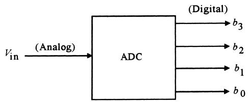
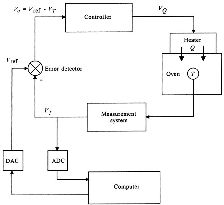
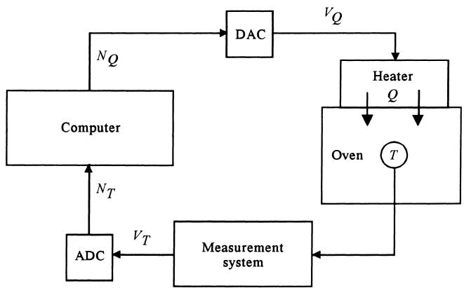
4. Describe ADC/DAC roles and the structure of supervisory and direct digital control.
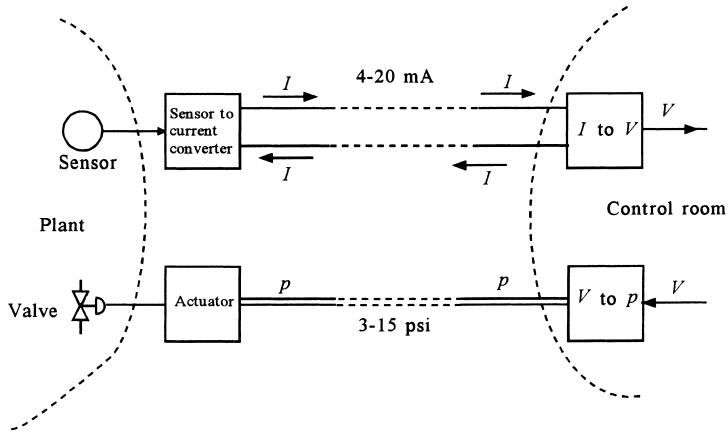
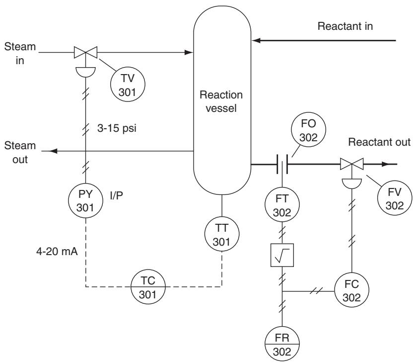
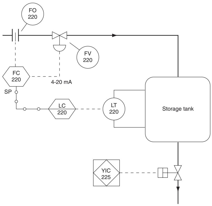
5. Interpret basic process-control drawings (P&IDs) and standard signal conventions (4–20 mA, 3–15 psi).
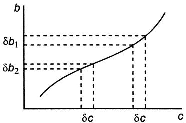
6. Use SI and English units, metric prefixes, and define accuracy, sensitivity, hysteresis, resolution, and linearity.

You don’t need to memorize every definition immediately, but you should come away being able to:

• Look at a control loop and talk about its performance in a structured way.
• Read an industrial diagram and understand what the signals and boxes mean.
• Do quick back-of-the-envelope checks involving units, percent error, and resolution.

Roadmap

1. Control System Evaluation
   • Error and control objectives
   • Stability, steady-state, transient response
   • Damped and cyclic criteria (minimum area, quarter amplitude)
2. Analog & Digital Processing
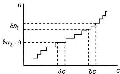
   • Analog vs digital data
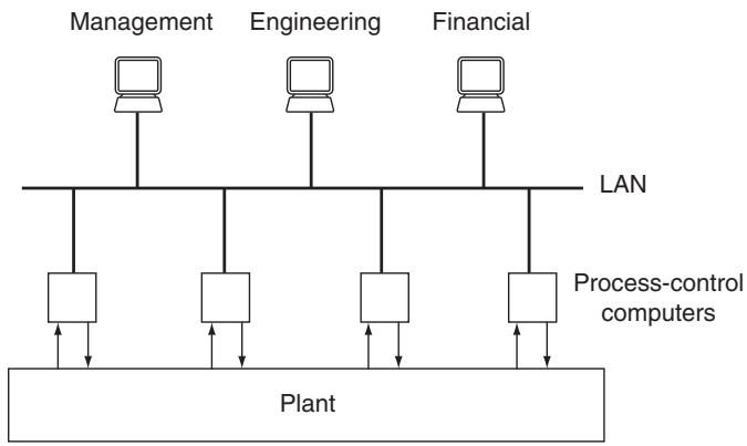
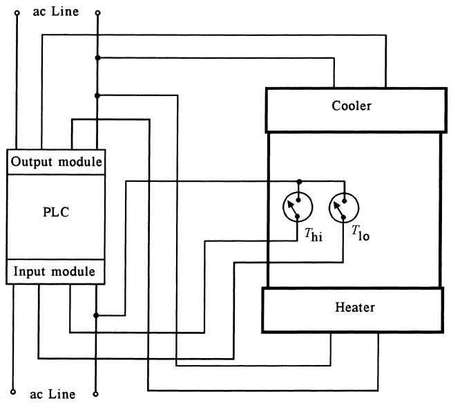
   • ON/OFF, analog, and digital control (supervisory, DDC, smart sensors, fieldbus)
3. Units & Standards in Process Control
   • SI base units, metric prefixes, conversions
   • 4–20 mA and pneumatic standards
   • Accuracy, resolution, linearity, P&IDs

Use the roadmap slide to frame the lecture as three big ideas. Students often already know a bit about PID and ADCs from prior courses; tie that prior knowledge explicitly to the new process-control context.

4 Control Error and Objective

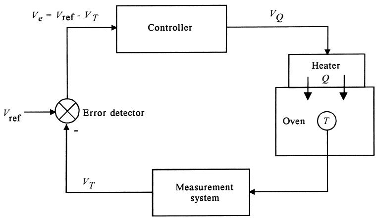
The basic performance variable in feedback control is the error:

\[ e(t) = r - c(t) \]

• \(r\): setpoint or reference (often constant, sometimes time-varying).
• \(c(t)\): controlled (measured) variable.
• \(e(t)\): difference between desired and actual value.

Ideal but impossible goal: make \(e(t) = 0\) for all \(t\).

Realistic goal: keep the error small enough and well-behaved in time for the process requirements.

Important

Three practical control objectives

1. The system must be stable.
2. It should have good steady-state regulation (small long-term error).
3. It should have good transient regulation (acceptable behavior during changes and disturbances).

Emphasize: controllers only act when there is an error. If the error were identically zero, the controller output would be constant and the loop would be pointless.

In real plants, “good enough” error is set by economic, safety, and quality constraints, not by math perfection.

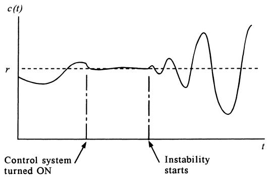
4.1 Stability – Why Controllers Can Make Things Worse

A controller changes the process input based on measurement feedback. If tuned improperly, this feedback can destabilize the process.

• Before control: output drifts randomly.
• After control is turned on: initially regulated near setpoint.
• Later: oscillations grow → instability caused by the control loop.

FIGURE 7: A control system can actually cause a system to become unstable.

Warning

Tightening control (increasing gain, making it more aggressive) usually improves performance up to a point, then dramatically increases instability risk.

Draw an analogy with driving a car: over-correcting steering at high speed leads to increasing swerves and possibly a crash.

Stability is the first objective: if it’s unstable, nothing else matters.

Interactive: Visualizing an Unstable Response

Ask students to edit the gain k and re-run:

• Small k → slow but stable.
• Larger k → faster response, then overshoot and possible divergence.

This simple discrete-time model mimics how aggressive control can trigger oscillations or blow-up.

4.2 Steady-State Regulation

Steady-state regulation focuses on the long-term error after all transients die out.

• Goal: minimize steady-state error.
• Often specified as an allowable band around setpoint: \(\pm \Delta c\).

Example:

• Target temperature: \(150^{\circ}\text{C}\).
• Allowable variation: \(\pm 2^{\circ}\text{C}\).
• Acceptable range: \(148^{\circ}\text{C} \le c(t) \le 152^{\circ}\text{C}\).

If the output drifts beyond this band, the control system must act to bring it back.

Tip

Steady-state performance is usually improved by integral action in a PID controller, but at the cost of slower transients or increased oscillation risk.

Point out that process engineers choose \(\Delta c\) based on product tolerance, energy cost, and safety. Steady-state performance is not just a math nicety; it dictates waste, off-spec product, and energy efficiency.

4.3 Transient Regulation

Transient regulation describes how the controlled variable behaves during sudden changes:

• Setpoint changes (e.g., jump from \(150^{\circ}\text{C}\) to \(160^{\circ}\text{C}\)).
• Disturbances (e.g., inlet flow or ambient temperature suddenly changes).

Key questions:

• How fast does the system reach the new setpoint?
• How big is the maximum error (overshoot or undershoot)?
• Does it ring/oscillate, and how long until it “settles”?

Note

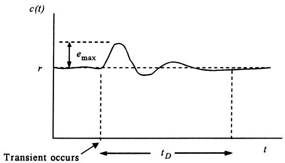
Transient response is usually characterized by:

• Duration \(t_D\) (rise/settling time).
• Maximum error \(e_{\max}\).
• Whether the response is damped or cyclic/oscillatory.

Connect to earlier control courses: these correspond to time-domain specs like rise time, peak time, percent overshoot, and settling time for second-order systems.

Here, though, the textbook uses a slightly different but conceptually equivalent notation \(t_D, e_{\max}\).

4.4 Evaluation Criteria – Big Picture

How do we judge how “good” a control loop is?

1. Stability:
   • Output remains bounded for bounded inputs.
   • No growing oscillations or runaway behavior.
2. Steady-State Response:
   • How small is the long-term error?
   • How well does it stay within the allowable band?
3. Transient Response:
   • How does it respond to setpoint steps and disturbances?
   • Tradeoff between speed (short \(t_D\)) and overshoot (small \(e_{\max}\)).

4.4 Evaluation Criteria – Big Picture

Tuning = adjusting controller parameters (e.g., PID gains) to balance these aspects.

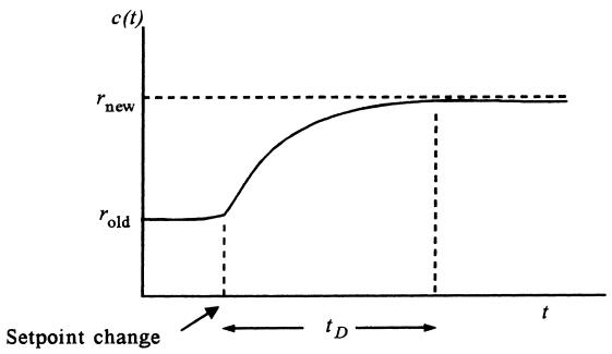
FIGURE 8a. Damped response to setpoint change

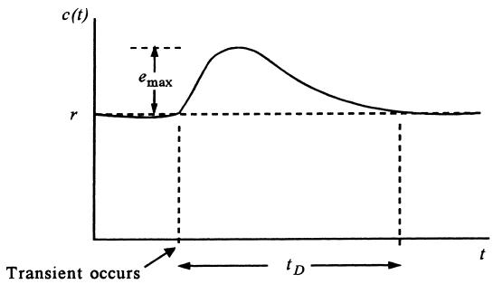
FIGURE 8b. Damped response to transient disturbance.

Emphasize that “best” tuning is context-dependent: e.g., a chemical reactor might accept slower response to reduce temperature overshoot (safety), whereas a robotic arm might favor speed.

Damped Response Criteria

In damped response, the error does not change sign; it approaches the setpoint monotonically.

Key metrics:

• Duration \(t_D\):
  • For a setpoint change: time for output to go from 10% to 90% of the total change.
  • For a disturbance: time from the start of disturbance until output is within 4% of reference.
• Maximum error \(e_{\max}\):
  • Peak deviation from the reference during the transient.

Different tuning → different \((e_{\max}, t_D)\) pairs for the same input.

Tip

Process designers must choose a compromise:

• Smaller \(e_{\max}\) but longer \(t_D\), or
• Larger \(e_{\max}\) but shorter \(t_D\).

Ask students: “If you’re designing temperature control for a sensitive semiconductor furnace, which do you prioritize: smaller overshoot or faster settling?”

Get them to articulate tradeoffs explicitly; this will foreshadow design exercises later in the course.

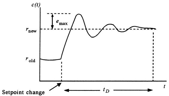
Cyclic (Underdamped) Response

Sometimes the desired response is allowed to oscillate around the setpoint.

In cyclic response:

• Output oscillates about reference.
• Parameters of interest:
  • Maximum error \(e_{\max}\).
  • Duration / settling time \(t_D\):
    • From when error first exceeds allowable band
    • To when it returns within the band and stays there.

Again, tuning adjusts the balance between overshoot and speed.

FIGURE 9a: Setpoint change oscillations.

FIGURE 9b: Transient change oscillations.

Relate this to standard second-order underdamped responses (ζ < 1).

In many industrial loops, mild oscillations are acceptable or even preferred, as long as they are decaying and within tolerance.

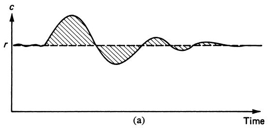
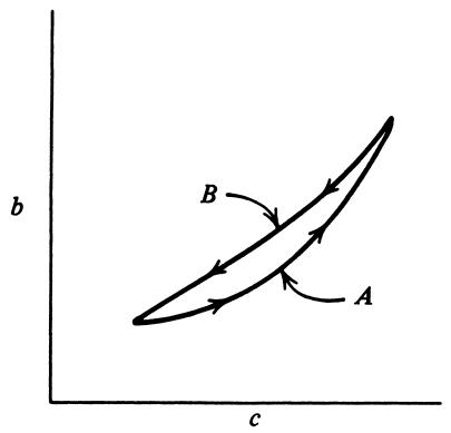
Cyclic Tuning Criteria: Minimum Area and Quarter Amplitude

Two common criteria for oscillatory responses:

1. Minimum-area criterion
   • Minimize area under \(|e(t)|\) vs. time curve: \[ A = \int |e(t)|\,dt = \text{minimum} \]
   • Intuitively: minimize “total error energy” during the transient.
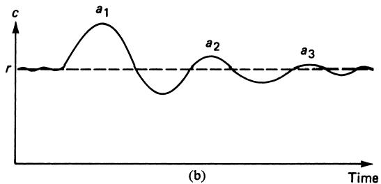
2. Quarter-amplitude criterion
   • Each peak is 1/4 of the previous: \[ a_2 = \frac{a_1}{4},\quad a_3 = \frac{a_2}{4}, \dots \]
   • Provides a specific underdamped oscillation pattern – reasonably fast decay with some overshoot.

FIGURE 10a. Minimum-area criteria.

FIGURE 10b. Quarter-amplitude criteria.

These criteria are historically used for hand-tuning PID controllers without full modeling.

In modern design, you might optimize a cost function numerically, but these rules still show up on plant floors as “rules of thumb.”

Problem Example: Choosing a Response

Scenario: You are tuning a temperature loop. A step change in setpoint causes the following:

• Tuning A:
  • \(e_{\max} = 8^{\circ}\text{C}\), \(t_D = 1.0\ \text{min}\).
• Tuning B:
  • \(e_{\max} = 2^{\circ}\text{C}\), \(t_D = 4.0\ \text{min}\).

Specification: maximum allowable deviation is \(\pm 3^{\circ}\text{C}\).

Question: Which tuning is acceptable, and which would you choose if you must also keep product quality high?

Solution Walkthrough

1. Check specification:
   • Allowable deviation ±3°C from setpoint.
2. Evaluate Tuning A:
   • \(e_{\max} = 8^{\circ}\text{C} > 3^{\circ}\text{C}\).
   • Violates spec → unacceptable.
3. Evaluate Tuning B:
   • \(e_{\max} = 2^{\circ}\text{C} \le 3^{\circ}\text{C}\).
   • Meets spec, even though it is slower.
4. Choose Tuning B:
   • Better steady-state and transient within allowable band.
   • For product quality, overshoot and undershoot beyond tolerance are more damaging than slower settling.

Tip

Key lesson: Performance specs constrain tuning choices – sometimes you must accept slower response to maintain quality and safety.

Use this example to reinforce: Always start from the specification (allowed band, safety constraints) and work backwards to tuning.

5 Analog vs Digital Processing in Control

Historically:

• Controllers were analog electronic circuits using op-amps, resistors, capacitors → analog processing.
• Now, most controllers are implemented by digital computers / microcontrollers → digital processing.

Analog processing:

• Variables represented by continuous voltages/currents.

Digital processing:

• Variables represented as binary numbers (bits) in a computer.

We still use analog sensors/actuators, but internal control logic is often digital.

Remind students they’ve seen analog circuits (op-amp PID implementations) and digital control (microcontroller reading ADC and writing PWM).

Industrial process control is essentially the same, just at plant scale, with more safety and robustness.

5.1 Analog vs Digital Data Representation

Analog Data

• Smooth, continuous relationship between variable \(c\) and representation \(b\).
• Every small change \(\delta c\) produces a proportional change \(\delta b\).
• Can be linear or nonlinear.

FIGURE 11a: Analog relation \(b(c)\).

Digital Data

• Variable \(c\) represented by discrete numeric value \(n\) (binary).
• Limited resolution: many nearby \(c\) values map to the same \(n\).
• Small changes may produce no change in code until threshold is passed.

FIGURE 11b: Digital relation \(n(c)\).

Clarify that in modern systems, sensors usually output analog voltages/currents; then an ADC converts them to digital for processing.

Nonlinearity in analog representation can be compensated numerically by the digital controller.

Digital Encoding Example – 4 Bits for 0–15 V

Table 1: Decimal-binary-hex encoding (4 bits)

Voltage	Binary	Hex
0	0000	0h
1	0001	1h
2	0010	2h
3	0011	3h
4	0100	4h
5	0101	5h
6	0110	6h
7	0111	7h
8	1000	8h
9	1001	9h
10	1010	Ah
11	1011	Bh
12	1100	Ch
13	1101	Dh
14	1110	Eh
15	1111	Fh

Digital Encoding Example – 4 Bits for 0–15 V

• Range: 0–15 V, resolution = 1 V per LSB (Least Significant Bit).
• Any two voltages between 4 and 5 V will both be encoded as 0100.
• Cannot distinguish between 4.25 V and 4.75 V.

Note

Increasing number of bits increases resolution:

• 4 bits → 16 levels
• 8 bits → 256 levels
• 12 bits → 4096 levels

Highlight that resolution is inherently limited in digital representations. If your control algorithm needs finer granularity, you must choose more bits in ADC/DAC.

ADCs and DACs in Control Loops

FIGURE 12: Example of ADC converting voltage into 4-bit digital signal.

• ADC (Analog-to-Digital Converter):
  • Converts analog sensor output (e.g., voltage) into digital code for the computer. ⭢ ADC Chip
• DAC (Digital-to-Analog Converter):
  • Converts digital controller output into an analog voltage or current for actuators. ⭢ DAC Chip

In process control:

• Sensors → analog → ADC → computer → DAC → analog actuators (valves, heaters).

Remind students that in embedded systems, they often use ADCs and PWM as a DAC-equivalent to control motors or heaters.

In process plants, DAC outputs often drive 4–20 mA loops or I/P (current-to-pressure) converters.

5.2 ON/OFF Control – Basic Digital Behavior

FIGURE 13: Elementary ON/OFF temperature control system.

• Final control elements (heater/cooler) have only two states: ON or OFF.
• Controller output is effectively a single bit: 0 or 1.
• Sensor and signal conditioning are analog, but decision is digital: \[ V_e = K(V_{\text{ref}} - V) \]

5.2 ON/OFF Control – Basic Digital Behavior

This system exhibits:

• Deadband: range of temperature where neither heater nor cooler is ON.
• Hysteresis: behavior differs depending on whether temperature is rising or falling (due to relay pull-in vs release voltages).

Real-world examples: home thermostats, water heaters, many HVAC systems.

Explain deadband/hysteresis as features, not bugs: they prevent chattering (rapid ON/OFF cycling) around the setpoint, which would wear out relays and actuators.

Ask students to think about their car’s AC cycling behavior as a familiar example.

5.3 Analog Control – Continuous Action

FIGURE 14: Analog heater control with continuous output.

In true analog control:

• All variables are analog representations of physical quantities.
• Heater power \(Q\) is an analog function of excitation voltage \(V_Q\).
• Error signal \(E\) is analog: difference between reference \(V_{\text{ref}}\) and measured \(V_T\).

5.3 Analog Control – Continuous Action

Advantages:

• Smooth actuation (no abrupt ON/OFF).
• Can implement proportional, integral, derivative actions with continuous op-amp circuits.

Disadvantages:

• Component drift, noise, calibration over time.
• Less flexible compared to software changes in digital controllers.

Point out that analog PID controllers are still used in some legacy systems because they are simple, robust, and fail-safe in certain ways.

But modern systems usually emulate analog behavior digitally.

5.4 Supervisory vs Direct Digital Control

Supervisory Control

FIGURE 15: Supervisory computer monitoring analog loops.

• Analog loops (like Figure 14) still do the real-time control.
• Computer monitors multiple loops and adjusts setpoints via ADC/DAC.
• If computer fails, analog loops continue using last setpoints.

Direct Digital Control (DDC)

FIGURE 16: Direct digital control loop.

• Controller function implemented entirely in software.
• ADC reads process variable; controller computes output; DAC drives actuator.
• Analog loop is replaced by digital logic.

Historically, supervisory control was an intermediate step when computers were unreliable.

Today, with highly reliable embedded processors, DDC is dominant, often distributed across smart sensors and local controllers.

5.4 Smart Sensors and Networked Control

Smart Sensor:

• Sensor + signal conditioning + ADC + microcontroller + (optionally) DAC in one housing.
• May output:
  • 4–20 mA to a valve, or
  • Digital data over a fieldbus (industrial LAN).

5.4 Smart Sensors and Networked Control

Networked Control Systems:

FIGURE 17: Local area network / fieldbus in process plant.

• Multiple DDC (Direct Digital Control) units distributed around plant.
• All connected via fieldbus (industrial LAN).
• Higher-level computers for:
  • Supervisory control, optimization, scheduling, accounting, etc.

Common standards: Foundation Fieldbus [US], Profibus [EU].

Relate to general networking knowledge: Ethernet, CAN (Controller Area Network) bus, etc.

Fieldbus is basically standardized industrial “plug and play” for process instruments: ensures multi-vendor interoperability.

5.5 Programmable Logic Controllers (PLCs)

• Programmable Logic Controllers (PLCs) evolved from electromechanical relay logic.
• Designed to control discrete-state devices: conveyors, valves, motors (ON/OFF).
• Programmed using ladder logic, function blocks, or structured text.

Modern PLCs can:

• Implement DDC for analog loops.
• Interface with smart sensors and fieldbus networks.

Programmable Logic Controllers (PLCs)

FIGURE 18: PLC-based ON/OFF control for heater/cooler.

In Figure 18:

• Thermal limit switches detect high/low temperature thresholds.
• PLC logic decides whether to energize heater or cooler (still ON/OFF).

Highlight that PLCs are ubiquitous in factories, water treatment plants, etc.

ECE students will likely encounter PLCs either directly or via protocols (Modbus, Profibus) in industrial automation roles.

6.1 Units in Process Control – SI and English

SI Base Units:

Quantity	Unit	Symbol
Length	meter	m
Mass	kilogram	kg
Time	second	s
Electric current	ampere	A
Temperature	kelvin	K
Amount of substance	mole	mol
Luminous intensity	candela	cd
Plane angle	radian	rad
Solid angle	steradian	sr

6.1 Units in Process Control – SI and English

Process-control engineers must fluently convert between:

• SI (Système International) units.
• English and other legacy units (CGS, etc.).

Derived units (examples):

• Force: newton \(1\ \text{N} = 1\ \text{kg·m/s}^2\).
• Energy: joule \(1\ \text{J} = 1\ \text{kg·m}^2/\text{s}^2\).
• Pressure: pascal \(1\ \text{Pa} = 1\ \text{N/m}^2\).

Industrial practice in the US is still full of psi, °F, gallons per minute, and feet.

Make sure students are comfortable mapping between those and SI units; show that equations are much cleaner in SI.

Worked Example – Pressure Unit Conversion

Example: Express \(p = 2.1 \times 10^{3}\ \text{dyne/cm}^2\) in pascals.

We know:

• \(10^2\ \text{cm} = 1\ \text{m}\).
• \(10^5\ \text{dyne} = 1\ \text{N}\).

So:

\[ p = \left(2.1 \times 10^{3}\ \frac{\text{dyne}}{\text{cm}^2}\right) \left(10^{2}\ \frac{\text{cm}}{\text{m}}\right)^2 \left(\frac{1\ \text{N}}{10^{5}\ \text{dyne}}\right) \]

Compute:

• \((10^2)^2 = 10^{4}\).
• \(2.1 \times 10^{3} \times 10^{4} / 10^{5} = 2.1 \times 10^{2} = 210\).

So:

\[ p = 210\ \frac{\text{N}}{\text{m}^2} = 210\ \text{Pa} \]

Stress dimensional analysis: always keep track of units in each step; if the final units are N/m², you’re at Pa by definition.

Metric Prefixes – Handling Very Large and Very Small Numbers

To simplify scientific notation, SI uses standard prefixes:

• \(10^{-6}\): micro (µ)
• \(10^{-3}\): milli (m)
• \(10^{3}\): kilo (k)
• \(10^{6}\): mega (M)
• \(10^{9}\): giga (G), etc.

Example: Express the following using decimal prefixes:

1. \(0.0000215\ \text{s}\)
2. \(3\,781\,000\,000\ \text{W}\)

Solution:

1. \[ 0.0000215\ \text{s} = 21.5 \times 10^{-6}\ \text{s} = 21.5\ \mu\text{s} \]

2. \[ 3\,781\,000\,000\ \text{W} = 3.781 \times 10^{9}\ \text{W} = 3.781\ \text{GW} \]

Metric prefixes show up constantly in instrumentation specs: kPa, mA, µV, Gbps.

Encourage students to mentally map between scientific notation and prefixes.

6.2 Analog Transmission Standards: 4–20 mA

FIGURE 19: Current and pneumatic signals in a plant.

Most common electrical transmission standard: 4–20 mA.

• E.g., temperature range 20–120°C encoded as 4–20 mA.
• 20°C → 4 mA; 120°C → 20 mA.
• 0 mA typically used to indicate fault (broken wire, device failure).

Analog Transmission Standards: 4–20 mA

Why current instead of voltage?

FIGURE 20: Current nearly independent of line resistance.

• Current loop is almost independent of wire resistance (0–1000 Ω).
• Voltage at receiver can vary, but as long as current is correct, the signal is accurate.

Highlight that many industrial transmitters are “two-wire” 4–20 mA devices: same two wires supply power and carry the signal.

Students should recognize 4–20 mA as a “universal language” of analog instrumentation.

Example – 4–20 mA Temperature Mapping

Example 7:

Temperature range: 20–120°C mapped linearly to 4–20 mA.

Find:

1. Current for \(T = 66^{\circ}\text{C}\).
2. Temperature corresponding to \(I = 6.5\ \text{mA}\).

Derive linear relation:

Assume \(I = mT + I_0\).

At \(T = 20^{\circ}\text{C}\), \(I = 4\ \text{mA}\):

\[ 4 = 20m + I_0 \]

At \(T = 120^{\circ}\text{C}\), \(I = 20\ \text{mA}\):

\[ 20 = 120m + I_0 \]

Example – 4–20 mA Temperature Mapping

Subtract:

\[ 16 = 100m \Rightarrow m = 0.16\ \text{mA}/^{\circ}\text{C} \]

Then:

\[ I_0 = 4 - 20 \cdot 0.16 = 0.8\ \text{mA} \]

So:

\[ I = 0.16 T + 0.8 \]

1. For \(T = 66^{\circ}\text{C}\):

\[ I = 0.16 \cdot 66 + 0.8 = 11.36\ \text{mA} \]

2. For \(I = 6.5\ \text{mA}\):

\[ 6.5 = 0.16 T + 0.8 \Rightarrow T = \frac{5.7}{0.16} = 35.6^{\circ}\text{C} \]

Encourage students to recognize this as a generic mapping problem: any linear sensor scaling can be handled the same way.

Good exercise for instrumentation calibration and microcontroller code.

6.2 Pneumatic Signal Standard

In pneumatic systems (air pressure in pipes):

• Common standard (US): 3–15 psi.

• For SI: 20–100 kPa is an equivalent standard.

• A measured variable is converted to proportional air pressure.

• Pressure propagates down long pipes without requiring electricity.

Advantages:

• Intrinsically safe in explosive environments.
• Historically reliable before widespread electronics.

Mention that even in modern plants, pneumatic actuators remain common, but their setpoints are now often driven by I/P (current-to-pressure) converters controlled by DDC systems.

6.3 Key Instrumentation Definitions: Transfer Function and Error

FIGURE 21: Block with input x(t), output y(t), transfer function.

• Transfer function \(T(x, y, t)\): relationship between input \(x(t)\) and output \(y(t)\).
  • Static transfer function: when input is constant (no time variation).
  • Dynamic transfer function: when input/time variation matters (often differential equations).
  • Examples:
    • Static: Flow meter, \(Q = 119.5 \sqrt{\Delta p}\).
    • Dynamic: First-order lag, second-order system, etc. (later sections).
• Error in control context:
  • For measurements: difference between actual value and measured indication.
  • For control: difference between setpoint and measured controlled variable.

Make sure students understand that “transfer function” here is more general than the Laplace-domain concept; here it can simply be input–output relationships, static or dynamic.

6.3 Key Instrumentation Definitions: Accuracy

Accuracy describes maximum expected error in instrument output.

Common forms:

1. As a fixed value: e.g., ±2°C.
2. As % of full-scale (FS): e.g., ±0.5% FS on 0–5 V → ±0.025 V.
3. As % of span: e.g., ±3% of span on 20–50 psi → ±0.9 psi.
4. As % of reading: e.g., ±2% of reading at 2 V → ±0.04 V.

6.3 Key Instrumentation Definitions: Accuracy

Example 8:

Temperature sensor span: 20–250°C. Measurement \(= 55^{\circ}\text{C}\).

• Accuracy ±0.5% FS:
  • FS = 250°C → error = ±0.005 × 250 = ±1.25°C.
  • Actual temp: 53.75°C to 56.25°C.
• Accuracy ±0.75% of span:
  • Span = 250–20 = 230°C → error = ±0.0075 × 230 = ±1.725°C.
  • Actual temp: 53.275°C to 56.725°C.
• Accuracy ±0.8% of reading:
  • Error = ±0.008 × 55°C = ±0.44°C.
  • Actual temp: 54.56°C to 55.44°C.

Emphasize that these are different ways of quoting the same concept; be careful when comparing device specs, because ±1% FS can be very different from ±1% of reading.

6.3 System Accuracy – Combining Errors

Consider two cascaded blocks:

FIGURE 22: Uncertainties build up through blocks.

Output voltage:

\[ V \pm \Delta V = (K \pm \Delta K)(G \pm \Delta G) C \]

Approximating for small uncertainties:

\[ \frac{\Delta V}{V} \approx \pm \frac{\Delta K}{K} \pm \frac{\Delta G}{G} \tag{5} \]

So worst-case fractional error is the sum of individual fractional errors.

More realistic rms (root mean square) combination:

\[ \left[\frac{\Delta V}{V}\right]_{\text{rms}} = \pm \sqrt{\left(\frac{\Delta K}{K}\right)^2 + \left(\frac{\Delta G}{G}\right)^2} \]

6.3 System Accuracy – Combining Errors

Example 11:

• Transducer: \(10\ \text{mV} / (\text{m}^3/\text{s}) \pm 1.5\%\).
• Signal conditioning: \(2\ \text{mA/mV} \pm 0.5\%\).

Net transfer function: \(20\ \text{mA} / (\text{m}^3/\text{s})\).

Worst-case accuracy:

\[ \frac{\Delta V}{V} = \pm (0.015 + 0.005) = \pm 0.02 = \pm 2\% \]

RMS accuracy:

\[ \left[\frac{\Delta V}{V}\right]_{\text{rms}} = \pm \sqrt{0.015^2 + 0.005^2} \approx \pm 0.0158 \approx \pm 1.6\% \]

Encourage students to always check whether a spec (e.g., ±1%) is for a single device or the whole chain.

RMS error combination is common in datasheets and standards.

6.3 Sensitivity, Hysteresis, Resolution, Linearity

• Sensitivity: change in output per change in input.
  • Example: 5 mV/°C.
• Hysteresis: different output for same input depending on direction of change (up vs down).
  • Usually specified as % FS of max deviation between increasing and decreasing curves.

FIGURE 23: Hysteresis in a transfer curve.

6.3 Sensitivity, Hysteresis, Resolution, Linearity

• Resolution: smallest change in input that produces a measurable change in output.
  • Often % FS.
  • Example 12: 0–150 N range, 0.1% FS resolution → 0.15 N smallest measurable step.
• Linearity: closeness of actual transfer curve to a straight line.
  • Often specified as max deviation from best-fit straight line as % FS. (See Figure 24.)

FIGURE 24: Nonlinearity vs best-fit straight line (5% FS).

Clarify that hysteresis is predictable if you always approach from the same direction; random reproducibility errors are not.

Resolution in digital systems is tied to 1 LSB of ADC/DAC; in analog, it is limited by noise and signal conditioning.

6.4 Process-Control Drawings: P&ID Overview

Piping and Instrumentation Diagrams (P&IDs) show:

• Process equipment (tanks, reactors, pumps).
• Product flow lines (usually heavy lines).
• Instruments: sensors, transmitters, controllers, valves, PLCs, computers.
• Signal types: analog current, pneumatic, digital bus.

6.3 Process-Control Drawings: P&ID Overview

FIGURE 25: Sample P&ID section with temperature and flow control.

Standard: ANSI/ISA S5.1-1984 (R1992).

• Instrument symbols: circles, circles in boxes, with letter/number codes (e.g., TT/301).
• Line types indicate signal nature (4–20 mA, air pressure, digital).

Stress that being able to read P&IDs is like reading schematics in electronics.

The letter codes (T, F, L, P, etc.) and line types are a standard language across the process industry.

6.3 P&ID Examples – Signals and Controllers

FIGURE 25: Temperature and flow control with pneumatic loops.

• TT/301: temperature transmitter.
• TC/301: temperature controller (accessed from control room).
• PY/301: I/P (current-to-pressure) converter.
• FT/302: flow transmitter; FC/302: flow controller; FR/302: flow recorder.

6.3 P&ID Examples – Signals and Controllers

FIGURE 26: Cascade level–flow control with computers and PLC.

• LC/220: level controller in control room (computer).
• FC/220: flow control computer in field.
• YIC/225: PLC controlling a drain valve.
• Digital bus indicated by solid lines with small bubbles.

Briefly decode one full loop: e.g., in Figure 26, tank level measured by LT/220 → LC/220 computes a setpoint for FC/220 → FC/220 drives valve FV/220 to control flow and thus indirectly control level.

That is an example of cascade control, where the output of one controller is the setpoint of another.

Interactive: Simple ADC Resolution Calculator

viewof bits = Inputs.range([4, 16], {step: 1, value: 8, label: "ADC bits"})
viewof vmin = Inputs.range([0, 5], {step: 0.5, value: 0, label: "Vmin"})
viewof vmax = Inputs.range([1, 10], {step: 0.5, value: 5, label: "Vmax"})

Let students play with bit count and voltage range:

• Increasing bits shrinks 1 LSB (better resolution).
• Increasing span with fixed bits grows LSB (worse resolution).

Tie back to Example 7 and 4–20 mA conversion: equivalent concept when you digitize current.

Summary / Key Points

1. Control evaluation
   • Error \(e(t) = r - c(t)\) is central.
   • Three main objectives: stability, good steady-state regulation, and good transient regulation.
2. Response criteria
   • Damped vs cyclic responses.
   • Metrics: duration \(t_D\), maximum error \(e_{\max}\).
   • Cyclic tuning rules: minimum area, quarter amplitude.
3. Analog vs digital processing
   • Analog: continuous voltages/currents; can be nonlinear.
   • Digital: discrete codes; limited resolution; requires ADC/DAC.

Summary / Key Points

4. Control architectures
   • ON/OFF control: simplest, widely used; introduces deadband/hysteresis.
   • Analog control: continuous action using analog circuits.
   • Supervisory control vs DDC; smart sensors; fieldbus (Foundation Fieldbus, Profibus).
   • PLCs for discrete and DDC duties.
5. Units and instrumentation definitions
   • SI base units and metric prefixes; be comfortable converting.
   • Industrial standards: 4–20 mA, 3–15 psi (20–100 kPa).
   • Accuracy, sensitivity, hysteresis, resolution, linearity, and system accuracy (worst-case vs rms).
   • P&IDs as the schematic language of process control.

Use this slide to recap, then ask a few concept-check questions:

• “Why might 4–20 mA be preferred to 0–20 mA?”
• “What is the difference between ±1% FS and ±1% of reading?”
• “What is the advantage of supervisory control vs DDC?”

Formulas & Relationships Summary

Error in control loop:

\[ e(t) = r - c(t) \]

Minimum-area cyclic criterion:

\[ A = \int |e(t)|\,dt = \text{minimum} \]

Linear mapping example (current vs temperature):

• For mapping \(T\) to \(I\): \[ I = mT + I_{0} \]

Formulas & Relationships Summary

Combining transfer-function uncertainties:

• Approximate worst-case fractional uncertainty: \[ \frac{\Delta V}{V} \approx \pm\frac{\Delta K}{K} \pm \frac{\Delta G}{G} \tag{5} \]

• RMS combination: \[ \left[\frac{\Delta V}{V}\right]_{\text{rms}} = \pm \sqrt{\left(\frac{\Delta K}{K}\right)^2 + \left(\frac{\Delta G}{G}\right)^2} \]

Metric prefix usage examples:

\[ 0.0000215\ \text{s} = 21.5\ \mu\text{s} \]

\[ 3.781 \times 10^{9}\ \text{W} = 3.781\ \text{GW} \]

Formulas & Relationships Summary

Sensor and system example sensitivities:

• Temperature sensor: 5 mV/°C → resolution and accuracy relate voltage to temperature via: \[ \Delta T = \frac{\Delta V}{5\ \text{mV}/^{\circ}\text{C}} \]

Encourage students to keep a personal “formula card” for this course and add these to it.

Many later problems will assume familiarity with these mappings and uncertainty combinations.