Introduction to Process Control

Instrumentation 1.1

Imron Rosyadi

Learning Objectives

By the end of this session, you should be able to:

1. Define what a control system is in engineering terms.
2. Distinguish among process control, servomechanisms, and discrete-state control systems.
3. Identify and describe the main elements in a process-control loop: process, sensor, error detector, controller, final control element, actuator.
4. Interpret and sketch a basic process-control block diagram.
5. Explain key performance criteria: stability, steady-state regulation, and transient response.
6. Use basic quantitative criteria (e.g., error, settling time, minimum area, quarter-amplitude) to evaluate control performance.

Read objectives slowly; connect them explicitly to later topics in the course (PID control, sensor selection, PLCs, etc.).

Stress that you’ll revisit this same block diagram in many later lectures: once they really internalize it, a lot of control theory feels less abstract.

Human Progress and Control

Human technological progress has been driven by better ways to control the environment.

• Keeping room temperature at \(21^\circ\mathrm{C}\)
• Guiding spacecraft to Jupiter
• Manufacturing integrated circuits with nanometer precision

All these are examples of control systems:

Methods to force parameters in the environment to have specific values.

Note

Key Idea A control system is the collection of elements needed to ensure some variable behaves the way we want it to, despite disturbances.

Relate to common ECE experiences:

• Voltage regulators forcing output to 5 V.
• Clock generation circuits keeping frequency constant.
• Wi-Fi power control keeping signal within limits.

Make the connection that “process control” is the industrial version of these same ideas.

Natural vs Artificial Control

Control is not just a human invention.

• Biological systems use natural process control:
  • Body temperature regulation
  • Heart rate and blood pressure
  • Glucose level control

Engineering systems use artificial control:

• Initially: human operators read gauges and turn valves.
• Now: automatic control using instruments, electronics, computers.

Briefly ask students: “What’s an example of ‘natural control’ you know from biology?” to make the concept stick.

Then transition: we will now study the artificial analog of such regulation, focusing on industrial processes.

Process Control: Basic Objective

In process control, the objective is to regulate the value of some quantity.

• To regulate: keep a variable at a desired value despite disturbances.
• Desired value: reference value or setpoint, usually denoted \(r\).

Examples:

• Maintain tank level at \(H\).
• Maintain reactor temperature at \(150^\circ\mathrm{C}\).
• Maintain motor speed at 1500 rpm.

Important

Regulation ≈ “hold at a setpoint.”

Clarify vocabulary:

• “Regulation” vs “tracking” (which comes later with servomechanisms).
• Use notation: actual controlled variable \(c(t)\), setpoint \(r\).

Tell them: “By the end of the course, when you hear ‘regulate temperature at 150°C,’ you should immediately picture a loop with process, sensor, controller, actuator.”

Tank-Level Example: The Process

We start with a simple process: a tank with inflow and outflow.

• Inflow: \(Q_{\mathrm{in}}\)
• Outflow: \(Q_{\mathrm{out}}\)
• Liquid level (height): \(h\)

Given relation:

\[ Q_{\mathrm{out}} = K\sqrt{h} \]

• Higher level \(h\) → higher outflow \(Q_{\mathrm{out}}\).
• If \(Q_{\mathrm{out}} > Q_{\mathrm{in}}\): level drops.
• If \(Q_{\mathrm{out}} < Q_{\mathrm{in}}\): level rises.

Tank process: inflow, outflow, level h, desired level H

Figure 1: Objective is to regulate the level \(h\) to desired value \(H\).

Emphasize: for now, no controller, no human—just physics.

Mention units: - \(h\) in ft (height). - \(Q\) in gal/min. - \(K\) given in gal/min per \(\mathrm{ft}^{1/2}\).

They will later see how such nonlinear process relations affect controller design.

Self-Regulation of the Tank

This process is self-regulating.

• For some constant \(Q_{\mathrm{in}}\), the level \(h\) changes until \(Q_{\mathrm{out}} = Q_{\mathrm{in}}\).
• At that point, \(h\) stops changing (steady state).

However:

• The steady-state level is not necessarily the level we want.
• If \(Q_{\mathrm{in}}\) changes, the level changes to a new value.

Warning

Self-regulation ≠ Control to a specified setpoint. It just finds some equilibrium, not necessarily your desired \(H\).

Draw on the board:

1. Start with some initial \(h\).
2. Show how a mismatch in flows causes level to change over time.

Explain that many physical systems “settle” somewhere, but that doesn’t mean they are controlled in the sense needed for engineering specifications.

Example 1: Self-Regulation Calculation

Problem

The tank has the relation

\[ Q_{\mathrm{out}} = K\sqrt{h} \]

with

• \(h\) in ft,
• \(K = 1.156\;(\mathrm{gal/min})/\mathrm{ft}^{1/2}\),
• Inflow \(Q_{\mathrm{in}} = 2\;\mathrm{gal/min}\).

At what value of \(h\) will the level stabilize due to self-regulation?

Example 1: Solution

At steady state (self-regulation):

\[ Q_{\mathrm{out}} = Q_{\mathrm{in}} \] So

\[ 2 = 1.156\sqrt{h} \] Solve for \(h\):

\[ h = \left(\frac{Q_{\mathrm{out}}}{K}\right)^2 = \left(\frac{2\;\mathrm{gal/min}}{1.156\;(\mathrm{gal/min})/\mathrm{ft}^{1/2}}\right)^2 \approx 3\;\mathrm{ft} \]

So the tank level will stabilize at 3 ft.

Note

This is a process property, not a controlled setpoint. If you changed \(Q_{\mathrm{in}}\), the self-regulated level would change.

Ask: “If I double \(Q_{\mathrm{in}}\), will \(h\) double?”

No—because \(Q_{\mathrm{out}} = K\sqrt{h}\), so \(h \propto Q_{\mathrm{in}}^2\).

Use this to highlight that the process may be nonlinear—a key issue for control design.

From Self-Regulation to Human Control

Suppose we want to maintain the level at a specific value \(H\), regardless of \(Q_{\mathrm{in}}\).

We add:

• A sensor to measure level, via a sight tube \(S\).
• A valve on the outlet to adjust \(Q_{\mathrm{out}}\).

The human strategy:

1. Read the actual level \(h\) on sight tube \(S\).
2. Compare \(h\) to the target level \(H\).
3. If \(h > H\): open valve → \(Q_{\mathrm{out}}\) increases → level falls.
4. If \(h < H\): close valve → \(Q_{\mathrm{out}}\) decreases → level rises.
5. Repeat small adjustments to keep level near \(H\).

Human regulating tank level via sight tube and valve

Figure 2: Human-aided level control using a sight tube and valve.

Point out roles:

• Controlled variable: tank level \(h\).
• Manipulated (controlling) variable: valve opening → affects \(Q_{\mathrm{out}}\).
• Sensor: sight tube.
• Controller: human brain.
• Control element: valve.

Ask them to imagine a water tank in a lab and how they would manually keep level constant.

From Human to Automatic Control

To automate, we replace the human with instruments.

Automatic system elements:

• Sensor: measures level and outputs signal \(s\) (voltage, current, pressure).
• Controller: electronic or computer-based device that:
  • Receives measurement \(s\),
  • Knows the setpoint \(H\),
  • Computes control signal \(u\).
• Actuator + Valve: receive \(u\) and adjust outflow.

Automatic level control with sensor, controller, actuator, valve

Figure 3: Automatic level-control system replacing the human.

When such automatic control is applied to processes, we call it process control.

Stress that the logic of the task hasn’t changed—only who/what does it.

Point to the idea of feedback: the sensor measures output, which is compared to setpoint, and the result is fed back to change the input.

Connect this to ECE language:

• Sensor output \(s\) might be a 4–20 mA signal.
• Controller might be a microcontroller running PID logic.

Servomechanisms vs Process Control

Another key class of control systems: servomechanisms.

• Objective: make a variable follow a time-varying reference.
• This is tracking control, not just regulation to a constant setpoint.

Example: Robot arm motion from point \(A\) to point \(B\).

Servomechanism traits:

• Controlled variable: position, angle, velocity, etc.
• Reference \(r(t)\) is a trajectory over time.
• Controller forces actual motion to follow \(r(t)\).

Robot arm moving from A to B using servomechanisms

Figure 4: Servomechanism-based robot arm control.

Note

Process control: keep variable near constant setpoint.
Servomechanism: make variable track a varying reference.

Help them map this to ECE:

• DC/BLDC motor position control in robotics → servomechanism.
• Power supply voltage regulation → process control.

Mention that although this book focuses on process control, many concepts overlap with servo control (feedback, stability, etc.).

Discrete-State Control Systems

Discrete-state control: controls sequences of events (on/off, start/stop).

Example: Paint manufacturing sequence:

1. Fill tank to a certain level.
2. Heat mixture to set temperature (with a temperature control loop).
3. Maintain temperature for a set time.
4. Start pump to transfer to next tank.
5. Start mixer; mix for specified duration.

Each step is: On or off, true or false, started or stopped.

These systems are:

• Often implemented using PLCs (Programmable Logic Controllers).
• Described using ladder logic, state machines, etc.

Stress that in a real plant, both types of control coexist:

• Continuous loops (flow, temperature, pressure).
• Discrete sequencing (start heater, open valve, alert alarm).

Tie to digital design: discrete-state control is similar to synchronous state machines, only with real-world actuators.

Generic Process-Control System Elements

To study control systems in a general way, we identify functional elements:

1. Process / Plant
2. Measurement (Sensor + Conditioning)
3. Error Detector
4. Controller
5. Control Element (Final Control Element)
6. Actuator

We’ll see how these appear in a block diagram, independent of the physical details.

Prepare to show Figure 5 and explicitly map each block to the tank-level example.

Use consistent notation:

• (\(c\)) controlled variable,
• (\(u\)) manipulated variable (control input to process),
• (\(r\)) setpoint,
• (\(b\)) measured value,
• (\(e\)) error.

Element 1: Process (Plant)

• The process (or plant) is what we’re trying to control.
• In the tank example:
  • Tank, fluid, inlet/outlet pipes, and their dynamics.

General characteristics:

• May involve many variables (temperature, pressure, flow, composition).
• May be:
  • Single-variable process (control one main variable), or
  • Multivariable process (several interrelated variables).

Note

In ECE, “plant” could be a motor, a DC-DC converter, an antenna system, etc.

Underline: in control theory, we often model the plant by differential equations or transfer functions.

Students will later learn how to derive simple models and how their structure affects stability and performance.

Element 2: Measurement & Sensor

To control a variable, we must measure it.

Measurement:

• Conversion of physical variable → analog signal:
  • Pneumatic pressure,
  • Electrical voltage/current,
  • Digital code.

Sensor: device that performs the initial measurement and energy conversion.

• Example: level sensor converting height to 4–20 mA.

Note

All sensors are transducers, but not all transducers are sensors.

• Sensor: physical variable → signal.
• Transducer (general): any signal form → another signal form.

Give some instrumentation examples:

• Thermocouple: temperature → voltage.
• Strain gauge: strain → resistance → voltage.
• Pressure transmitter: pressure → 4–20 mA.

Explain “signal conditioning” (amplification, filtering, linearization) that usually follows the raw sensor.

Element 3: Error Detector

We compare the setpoint \(r\) to the measured value \(b\).

• Error signal:

\[ e = r - b \]

• \(e\) has magnitude and sign (polarity).

Although often embedded inside the controller, we conceptually separate it as:

• A summing junction or subtractor.

Important

Error is the core quantity the controller reacts to.

Relate to the human example:

• Human mentally computes “am I above or below the desired level?”

Later, when doing block diagrams, show the \(\oplus\) symbol with incoming arrows \(r\) and \(-b\), output \(e\).

Element 4: Controller

The controller receives the error \(e\) and decides how to act.

Roles:

• Evaluate error over time.
• Output control signal \(p\) (or \(u\), depending on notation) to drive the process.

Implementation forms:

• Human operator (early systems).
• Pneumatic or analog electronic circuits.
• Digital controllers: microprocessors, PLCs, embedded systems.

Typical controller logic: Proportional (P), Integral (I), Derivative (D) actions → PID control.

Tip

The controller “translates” error into an appropriate manipulation of the process.

Stress that in modern process control, controllers are increasingly software running on industrial computers or PLCs.

Mention that tuning the controller (choosing gains, time constants) is a key engineering decision.

Element 5: Control Element & Actuator

Final Control Element (Control Element):

• The device that directly influences the process variable.
• Examples:
  • Control valve.
  • Variable-speed drive for a motor.

Actuator:

• Intermediate device converting controller’s low-energy signal → physical action.
• Examples:
  • Motorized valve operator.
  • Power electronics controlling a motor.

Note

Actuator: small signal in → big energy out.

Map to ECE:

• DAC or PWM output from microcontroller → gate driver → MOSFET bridge → motor.
• Controller output (= small electronic signal) can’t by itself turn a large valve or motor.

Clarify that in some small systems, actuator and final control element might be integrated as one device.

Generic Process-Control Block Diagram

Figure 5: Generic block diagram of a feedback control loop

Signals:

• \(r\): reference (setpoint).
• \(c\): controlled variable (process output).
• \(b\): measured value (feedback signal).
• \(e = r - b\): error.
• \(p\): controller output to control element.
• \(u\): manipulated variable into process.

Walk through the loop slowly:

1. Setpoint \(r\) enters the summing junction.
2. Measured value \(b\) is subtracted → error \(e\).
3. Controller converts \(e\) into output \(p\).
4. Control element (valve, etc.) converts \(p\) into manipulated variable \(u\).
5. Process converts \(u\) into controlled output \(c\).
6. Measurement block converts \(c\) into \(b\) for feedback.

Stress: This loop is the canonical picture of feedback control.

Example: Flow-Control Loop (Physical vs Block Diagram)

Physical system

Physical diagram of flow control loop

Block diagram abstraction

Block diagram of the same control loop

Example: Flow-Control Loop (Physical vs Block Diagram) (cont.)

Physical system

1. Physical flow control loop:

• Orifice plate (creates differential pressure).
• \(\Delta P\) transmitter → 3–15 psi signal.
• P/I converter → 4–20 mA to controller.
• Controller output: 4–20 mA.
• I/P converter → 3–15 psi to actuator.
• Pneumatic actuator → control valve.

Block diagram abstraction

2. Block diagram:

• Measurement block: Orifice, transmitter, P/I.
• Controller block.
• I/P, actuator, valve as control element.
• Process: pipe flow system.

Highlight that in the physical view, many intermediate transducers (P/I, I/P) appear.

The block diagram view groups these into functional blocks to simplify analysis.

Tie to ECE instrumentation: 4–20 mA is robust for industrial noise, long cable runs; 3–15 psi was used widely in older pneumatic systems.

The Feedback Loop Concept

Notice the closed path of signals in Figure 5:

1. Process output \(c\) is measured as \(b\).
2. Error \(e = r - b\) is computed.
3. Controller adjusts input \(u\) to process.
4. Process output changes, and the cycle repeats.

This is a feedback loop.

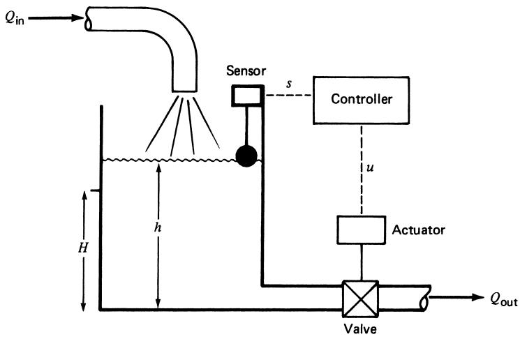
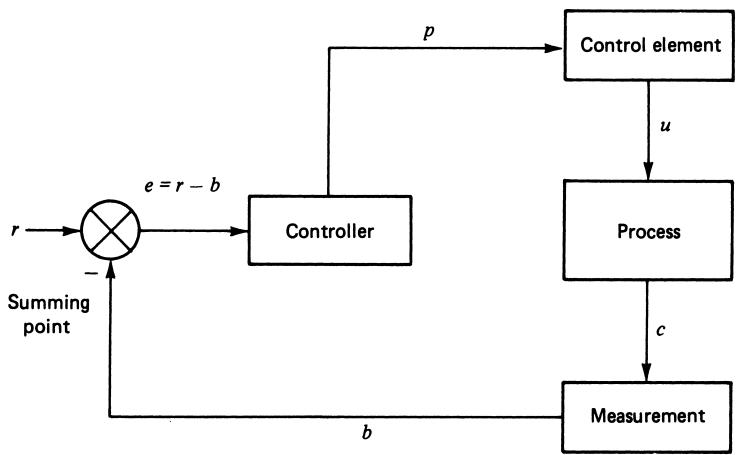
• The system uses information about its output to continuously correct itself.

Important

A process-control loop is typically a feedback loop. Feedback can both improve performance and cause instability if misused.

Explain that feedback is a powerful concept appearing in many domains:

• Electronic amplifiers (negative feedback).
• Control of drones and robots.
• Biological systems (hormone regulation).

Mention that later in the course, they’ll study stability criteria and frequency-domain analysis for such loops.

Evaluating Control System Performance

We now ask: How well is the control system working?

We use error as the performance measure:

\[ e(t) = r - c(t) \]

Three main objectives:

1. Stability
2. Good steady-state regulation
3. Good transient regulation

Tuning the control loop = adjusting it to balance these objectives.

Emphasize: there is no free lunch—better steady-state performance often comes at the cost of worse transient behavior or reduced stability margin.

They will later see how tuning PID gains shapes this tradeoff.

Objective 1: Stability

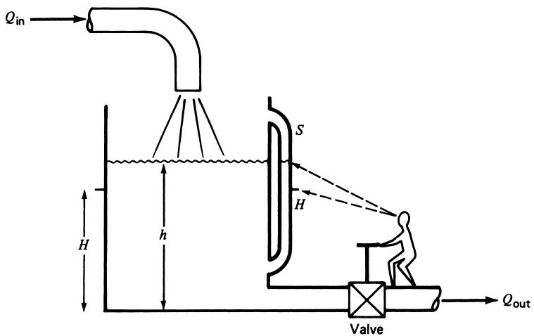
• Purpose of control: regulate a variable by acting on the process.
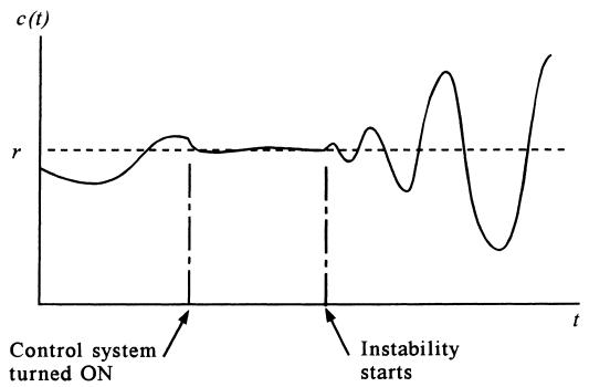
• If the controller acts too aggressively or incorrectly, it can cause instability.

Figure 7: Initially, uncontrolled drift. After control is turned on, variable moves to setpoint, then later develops growing oscillations due to instability.

Warning

A control system can cause a system to become unstable. Tight control (fast response) often risks instability.

Ask: “Does adding control always make a system better?” Then show the figure—answer: not necessarily.

Relate to audio feedback (microphone + speaker “howl”): that’s an unstable loop.

Later, they’ll learn about gain margins and phase margins as formal stability measures.

Objective 2: Steady-State Regulation

Steady-state regulation:

• How small is the error after transient effects die out?

Often specified as an acceptable band:

• Allowable deviation \(\pm \Delta c\) around setpoint.
• Example:
  • Setpoint \(150^\circ\mathrm{C}\).
  • Allowable band: \(148^\circ\mathrm{C} \le c \le 152^\circ\mathrm{C}\).

Goal: Minimize steady-state error while maintaining stability.

Note

Steady-state performance is about accuracy of long-term regulation.

Introduce the idea of offset: when the controlled variable settles at a value slightly different from setpoint.

Mention that integral action (I) in PID is often added to eliminate steady-state error, but again, this can worsen transient behavior.

Objective 3: Transient Regulation

Transient regulation asks: How does the system behave when a sudden change occurs?

Two main types of transients:

1. Setpoint change:
   • Example: change temperature setpoint from \(150^\circ\mathrm{C}\) to \(160^\circ\mathrm{C}\).
2. Disturbance/change in other variables:
   • Example: sudden change in inlet flow or feed composition.

Key questions:

• How large is the temporary deviation from desired value?
• How long does it take to return close to the setpoint?

This is often called the transient response.

Important

Good transient regulation = small overshoot and short time to settle.

Show simple sketches of good vs poor transient responses (even hand-drawn on whiteboard).

Make sure students understand:

• You can’t judge a controller just by its final value.
• The path it takes to get there (overshoot, oscillation) also matters.

Overall Evaluation Criteria

We evaluate a control system by:

1. Ensuring stability (no unbounded oscillations).
2. Assessing steady-state error (accuracy of long-term regulation).
3. Assessing transient response:
   • To setpoint changes.
   • To disturbances.

The process of adjusting the control loop to meet these criteria is called tuning.

State that later in the course they’ll learn practical tuning rules (e.g., Ziegler–Nichols, Cohen–Coon) and see how such rules implicitly target certain performance criteria (e.g., quarter-amplitude damping).

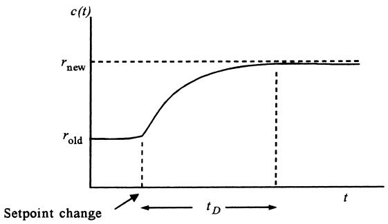
Damped (Overdamped) Response

In one tuning approach, we desire a damped response:

• Error does not oscillate around the setpoint.
• It moves in one direction toward the new value and stays there.

Measures:

• Duration \(t_D\):
  • For setpoint change: time from 10% to 90% of final change.
  • For transient: time from disturbance start until variable is within 4% of reference again.
• Maximum error \(e_{\max}\) during the transient.

Tradeoffs:

• You can get smaller \(e_{\max}\) at cost of larger \(t_D\), and vice versa.

Figure 8: Damped response to setpoint and transient changes

Explain:

• Faster response (small \(t_D\)) may cause larger peak error.
• Slower, more cautious response gives smaller overshoot but takes longer.

Relate to everyday experience—turning a steering wheel sharply vs smoothly.

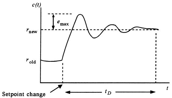
Cyclic (Underdamped) Responsea

Another tuning approach allows oscillatory (cyclic) transient response.

Measures:

• Maximum error \(e_{\max}\).
• Settling time \(t_D\): time from when error first exceeds allowable band until it returns within band and stays there.

Again, tuning changes:

• Number of oscillations.
• Amplitude of oscillations.
• Settling time.

Figure 9: Setpoint and disturbance responses with oscillations (cyclic response)

Warning

Cyclic response is acceptable only if oscillations are damped and stay within acceptable error limits.

Relate to second-order system responses in classical control: “underdamped” vs “overdamped.”

Mention that some oscillation can be acceptable if it results in faster settling than an overdamped response.

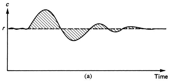
Quantitative Cyclic Criteria: Minimum Area & Quarter-Amplitude

Two standard cyclic tuning criteria:

Minimum Area Criterion

• Define error-area:

\[ A = \int |e(t)|\,dt \]

• Tune controller to minimize \(A\) for a given excitation.
• Interpreted as minimizing the total cumulative error over time.

Shaded region = area under \(|e(t)|\).

Quarter-Amplitude Criterion

• In oscillatory response, each peak amplitude is ¼ of the previous:

\[ a_2 = \frac{a_1}{4},\quad a_3 = \frac{a_2}{4},\ \dots \]

• Produces a quickly decaying oscillation.
• Historically popular in process control tuning (e.g., Ziegler–Nichols).

Minimum area and quarter-amplitude criteria

Figure 10: Minimum area and quarter-amplitude response shapes.

Explain what \(|e(t)|\) means—absolute value ensures positive contribution from both sides of the setpoint.

Point out that these criteria are sometimes more theoretical; in practice, engineers use trial, simulation, and experience but still think in terms of these tradeoffs.

Interactive Exercise: Explore a Simple First-Order Response

Use this interactive code block to see how a simple first-order system responds to a step change in setpoint.

Adjust time constant and gain to see how they affect speed and error.

viewof tau = Inputs.range([0.1, 10], {step: 0.1, value: 2, label: "Time constant τ"})
viewof k = Inputs.range([0.1, 5], {step: 0.1, value: 1, label: "Gain K"})

Explain that this is not yet a full feedback loop model, but a simple first-order response is often a decent approximation of many process-control loops near operating points.

Ask students to:

• Increase τ → see slower response.
• Increase K → see larger steady-state output.

Use this to prepare them for the idea of time constant and gain in dynamic models and how they impact tuning.

Summary / Key Points

1. Control systems force environmental or process variables to have desired values.

2. Process control focuses on regulating variables (like level, temperature, flow) to constant setpoints despite disturbances.

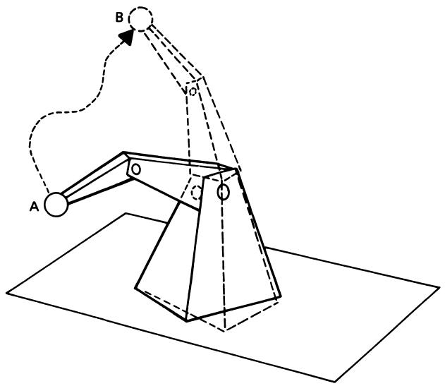
3. Servomechanisms perform tracking of time-varying references (e.g., robot arm motion).

4. Discrete-state control systems manage sequences of events (on/off, start/stop) and are often implemented using PLCs.

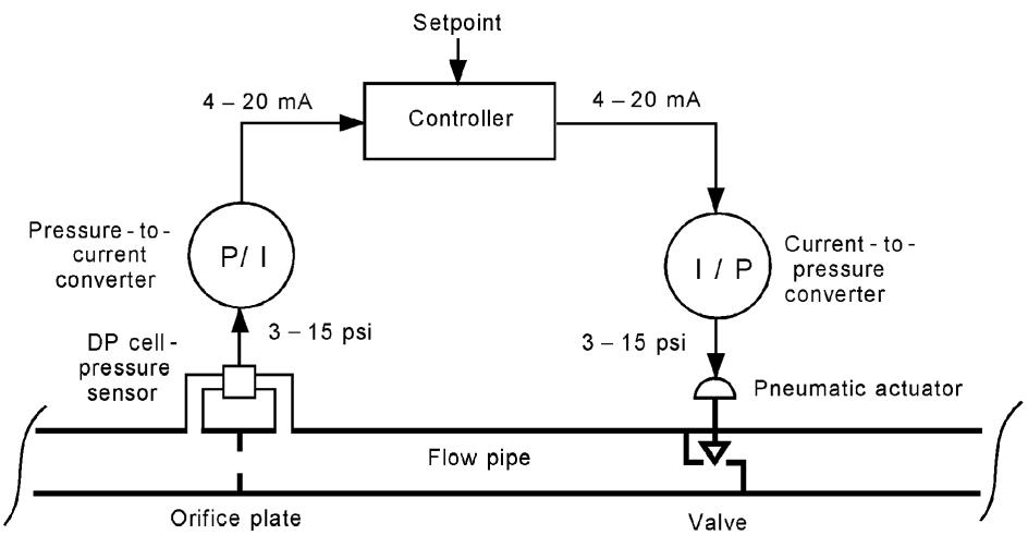
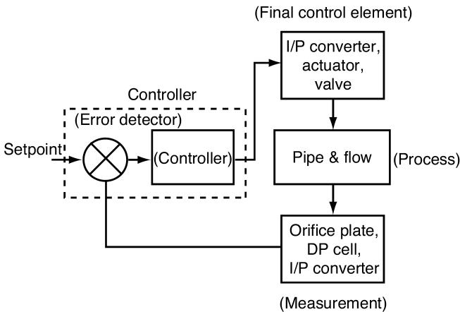
5. A generic process-control loop includes:

   • Process (plant).
   • Measurement & sensor.
   • Error detector \(e = r - b\).
   • Controller.
   • Control element (final control element) and actuator.

Summary / Key Points

6. The loop forms a feedback system, where measured output is used to adjust input.

7. Control performance is evaluated via:

   • Stability (no unbounded oscillations).
   • Steady-state regulation (small long-term error).
   • Transient response (overshoot, settling time).

8. Tuning adjusts controller parameters to trade off between speed, error magnitude, and stability, using criteria such as minimum area or quarter-amplitude decay.

Use this slide to recap and check understanding: ask students to identify the controlled, manipulated, and disturbance variables in a real-world example (e.g., home air-conditioner).

Encourage them to re-draw Figure 5 from memory as a mental framework.

Formula & Notation Summary

Key variables and formulas used in this session:

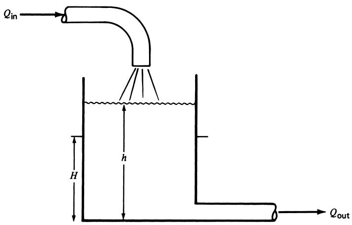
• Flow–level relation in tank:

\[ Q_{\mathrm{out}} = K\sqrt{h} \]

• Self-regulated level for given \(Q_{\mathrm{in}}\):

\[ Q_{\mathrm{out}} = Q_{\mathrm{in}} \Rightarrow h = \left(\frac{Q_{\mathrm{out}}}{K}\right)^2 \]

• Error definition:

\[ e(t) = r - c(t) \]

Formula & Notation Summary

• Minimum-area performance criterion:

\[ A = \int |e(t)|\,dt = \text{minimum} \]

• Quarter-amplitude criterion for cyclic response:

\[ a_2 = \frac{a_1}{4},\quad a_3 = \frac{a_2}{4},\ \dots \]

Remind students to be comfortable with this notation early in the course: \(r, c, b, e, u\).

They will see these symbols consistently in control textbooks and in subsequent lectures.