8.4 Infinite Impulse Response (IIR) Filter Design
Digital Signal Processing
8.9–8.12: What We’ll Focus On Today
Chapter topics covered in this session:
8.9 Application: 60‑Hz hum eliminator & heart‑rate detection in ECG
8.10 Coefficient accuracy effects on IIR filters
8.11 Application: DTMF generation & detection using the Goertzel algorithm
8.12 Summary & practical choice of IIR design methods
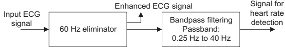
8.9 ECG: 60‑Hz Hum Eliminator – Why We Care
Problem context (ECE / biomedical):
ECG signals are very low‑amplitude (on the order of mV).
Power‑line interference (60 Hz in US, 50 Hz in many other countries) easily corrupts ECG traces.
Nonlinearities in electrodes and amplifiers can create harmonics at 120 Hz, 180 Hz, etc.
Severe interference can make the ECG unusable for diagnostics or even basic heart‑rate measurement.
Engineering target:
Remove 60 Hz + 120 Hz + 180 Hz components.
Preserve the clinically useful ECG content for:
General ECG analysis (0.01–250 Hz).
Heart‑rate detection (narrower band is enough).
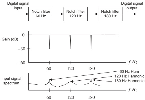
60‑Hz Hum Eliminator Concept
We cascade three second‑order IIR notch filters :
Notch 1: 60 Hz
Notch 2: 120 Hz
Notch 3: 180 Hz
Each notch:
Center (notch) frequency: \(f_0 \in \{60,120,180\}\) Hz
3‑dB bandwidth: 4 Hz
Sampling rate: \(f_s = 600\) Hz
Design method: pole‑zero placement
Combined response ≈ product of three notches.
Remind students: a notch filter places zeros on the unit circle at the hum frequency and nearby poles slightly inside the unit circle to control bandwidth. Cascading multiplies responses: deep notches at each harmonic while leaving most other frequencies relatively untouched.
The bandpass‑filtered ECG (0.25–40 Hz) is good for heart‑rate detection , but not for full diagnostic ECG analysis (which needs ≈0.01–250 Hz).
Designing One Notch Filter (60 Hz) – Geometry
For a second‑order digital notch filter:
Sampling rate: \(f_s=600\) Hz
Notch frequency: \(f_0=60\) Hz
Desired 3 dB bandwidth: 4 Hz
We choose a pole radius \(r < 1\) from:
\[
r = 1 - \frac{BW}{f_s}\pi = 1 - \frac{4}{600}\pi \approx 0.9791
\]
Normalized digital frequency (in degrees):
\[
\theta = \frac{f_0}{f_s}\times 360^\circ = \frac{60}{600}\times 360^\circ = 36^\circ
\]
Compute:
\(2\cos(36^\circ) = 1.6180\) \(2r\cos(36^\circ) = 1.5842\)
Gain scale factor \(K\) :
\[
K = \frac{1 - 2r\cos\theta + r^2}{2 - 2\cos\theta} \approx 0.9803
\]
Intuition: zeros at angle ±θ on the unit circle create the notch. Poles at radius r, slightly inside, sharpen the notch and control bandwidth. K normalizes overall gain so passband ≈ 0 dB.
60‑Hz Notch Filter – Transfer Function & Difference Equation
The 60‑Hz section:
\[
H_1(z) = \frac{0.9803 - 1.5862 z^{-1} + 0.9803 z^{-2}}{1 - 1.5842 z^{-1} + 0.9586 z^{-2}}
\]
Difference equation (input \(x(n)\) , output \(y_1(n)\) ):
\[
\begin{aligned}
y_1(n) &= 0.9803\,x(n) - 1.5862\,x(n-1) + 0.9802\,x(n-2) \\
&\quad + 1.5842\,y_1(n-1) - 0.9586\,y_1(n-2)
\end{aligned}
\]
Other two notch sections:
120 Hz section, input \(y_1(n)\) , output \(y_2(n)\) :
\[
H_2(z)=\frac{0.9794 - 0.6053 z^{-1} + 0.9794 z^{-2}}{1 - 0.6051 z^{-1} + 0.9586 z^{-2}}
\]
\[
\begin{aligned}
y_2(n) &= 0.9794\,y_1(n) - 0.6053\,y_1(n-1) + 0.9794\,y_1(n-2) \\
&\quad + 0.6051\,y_2(n-1) - 0.9586\,y_2(n-2)
\end{aligned}
\]
180 Hz section, input \(y_2(n)\) , output \(y_3(n)\) :
\[
H_3(z)=\frac{0.9793 + 0.6052 z^{-1} + 0.9793 z^{-2}}{1 + 0.6051 z^{-1} + 0.9586 z^{-2}}
\]
\[
\begin{aligned}
y_3(n) &= 0.9793\,y_2(n) + 0.6052\,y_2(n-1) + 0.9793\,y_2(n-2) \\
&\quad - 0.6051\,y_3(n-1) - 0.9586\,y_3(n-2)
\end{aligned}
\]
In implementation, you typically realize each second‑order section (“biquad”) separately and cascade them: \[
y_3(n) = H_3(z)\,H_2(z)\,H_1(z)\,x(n)
\]
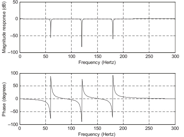
Frequency Response of the Cascaded Notches
Highlight: even though each biquad is simple, cascading gives strong rejection at the hum frequencies while minimally affecting most of the ECG band. Ask: what might happen if hum frequency drifts (e.g., 59.8 Hz)? This motivates bandwidth choice.
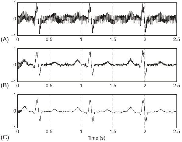
Stage 2: Bandpass Filter for Heart‑Rate Detection
After hum removal (\(y_3(n)\) ), we still see:
DC drift (very low frequency baseline wander).
Muscle noise, typically > 40 Hz.
We design a 4th‑order Chebyshev bandpass :
Passband: 0.25–40 Hz
Passband ripple: 0.5 dB
Design method: bilinear transform (BLT) from an analog prototype.
Sampling rate: \(f_s = 600\) Hz.
Resulting transfer function:
\[
H_4(z)=\frac{0.0464 - 0.0927 z^{-2} + 0.0464 z^{-4}}{1 - 3.3523 z^{-1} + 4.2557 z^{-2} - 2.4540 z^{-3} + 0.5506 z^{-4}}
\]
Difference equation (input \(y_3\) , output \(y_4\) ):
\[
\begin{aligned}
y_4(n) &= 0.0464\,y_3(n) - 0.0927\,y_3(n-2) + 0.0464\,y_3(n-4) \\
&\quad + 3.3523\,y_4(n-1) - 4.2557\,y_4(n-2) \\
&\quad + 2.4540\,y_4(n-3) - 0.5506\,y_4(n-4)
\end{aligned}
\]
Total zero crossings: sum over n.
Number of peaks ≈ half the zero crossings.
Heart rate estimation:
\[
HR = \frac{60}{\frac{N}{f_s}} \times \frac{\text{zero crossings}}{2}
\]
Heart‑Rate Example Calculation
In the example:
Data length: \(N=1500\) samples.
Sampling rate: \(f_s=600\) Hz.
Total zero crossings detected: 6.
Compute HR:
\[
\begin{aligned}
HR &= \frac{60}{\frac{1500}{600}} \times \frac{6}{2} \\
&= \frac{60}{2.5} \times 3 \\
&= 24 \times 3 = 72\ \text{beats per minute}.
\end{aligned}
\]
This is a crude detector but works reasonably well with a clean, band‑limited ECG. Modern systems rely on more sophisticated feature detection (e.g., QRS detectors).
8.10 Coefficient Accuracy Effects on IIR Filters
In practice:
Filter coefficients are quantized (finite word length), especially on fixed‑point DSPs.
Quantization moves pole and zero locations , changing frequency response and possibly stability.
General IIR form (first order):
\[
H(z) = \frac{b_0 + b_1 z^{-1}}{1 + a_1 z^{-1}}
\]
After quantization:
\[
H^q(z) = \frac{b_0^q + b_1^q z^{-1}}{1 + a_1^q z^{-1}}
\]
Poles and zeros:
\[
z_1 = -\frac{b_1^q}{b_0^q}, \qquad p_1 = -a_1^q
\]
Second‑order case:
\[
H(z) = \frac{b_0 + b_1 z^{-1} + b_2 z^{-2}}{1 + a_1 z^{-1} + a_2 z^{-2}}
\]
\[
H^q(z) = \frac{b_0^q + b_1^q z^{-1} + b_2^q z^{-2}}{1 + a_1^q z^{-1} + a_2^q z^{-2}}
\]
Zeros:
\[
z_{1,2} = -\frac{1}{2}\frac{b_1^q}{b_0^q} \pm j\left(\frac{b_2^q}{b_0^q} - \frac{1}{4}\left(\frac{b_1^q}{b_0^q}\right)^2\right)^{1/2}
\]
Poles:
\[
p_{1,2} = -\frac{1}{2} a_1^q \pm j\left(a_2^q - \frac{1}{4}(a_1^q)^2\right)^{1/2}
\]
Stress the connection between coefficient accuracy and pole radius: if a pole intended at r ≈ 0.99 gets quantized to r ≈ 1.01, the filter can become unstable. This motivates using second‑order sections and enough bits.
Example 8.24 – 1st‑Order IIR Quantization
Given ideal filter:
\[
H(z) = \frac{1.2341 + 0.2126 z^{-1}}{1 - 0.5126 z^{-1}}
\]
We have 1 sign bit + 6 magnitude bits = 7‑bit fixed‑point, with scaling chosen so max coefficient lies in [1,2).
Scale by \(2^5\) :
\(1.2341 \times 2^5 \approx 39.49 \rightarrow 39\) → \(b_0^q = 39/32 = 1.21875\) .Similarly:
\(b_1^q = 0.1875\) \(a_1^q = -0.5\)
Quantized transfer function:
\[
H^q(z) = \frac{1.21875 + 0.1875 z^{-1}}{1 - 0.5 z^{-1}}
\]
Poles and zeros (before vs. after):
Original zero: \(z_1 = -\frac{0.2126}{1.2341} \approx -0.1723\) .
Quantized zero: \(z_1^q \approx -\frac{0.1875}{1.21875} \approx -0.1538\) .
Original pole: \(p_1 = 0.5126\) .
Quantized pole: \(p_1^q = 0.5\) .
Even small coefficient rounding changes pole/zero positions, which changes magnitude and phase response. Here, changes are mild; but in high‑order filters, effects can accumulate.
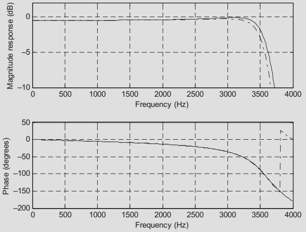
Example 8.25 – 2nd‑Order Chebyshev Lowpass
Original design (fs = 8 kHz, passband ripple 0.5 dB, \(f_c = 3.4\) kHz):
\[
H(z) = \frac{0.7434 + 1.4865 z^{-1} + 0.7434 z^{-2}}{1 + 1.5149 z^{-1} + 0.6346 z^{-2}}
\]
Quantization:
1 sign bit + 7 magnitude bits, scale factor \(2^6\) .
Quantized filter:
\[
H^q(z) = \frac{0.7500 + 1.484375 z^{-1} + 0.7500 z^{-2}}{1 + 1.515625 z^{-1} + 0.640625 z^{-2}}
\]
Poles/zeros (approx):
Unquantized zeros: \(-1, -1\) (double real zero at \(-1\) ).
Quantized zeros: \(-0.9896 \pm j 0.1440\) .
Unquantized poles: \(-0.7574 \pm j 0.2467\) .
Quantized poles: \(-0.7578 \pm j 0.2569\) .
Magnitude/phase comparison:
Solid: ideal coefficients.
Dash‑dotted: quantized.
Observation:
Magnitude response shows visible deviation, especially near cutoff.
Phase response in passband is less affected.
8.11 DTMF: Real‑World Telephony Application
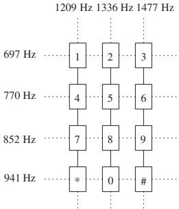
DTMF (Dual‑Tone Multi‑Frequency) :
Each telephone keypad key encodes two tones:
One from a low‑frequency group (rows).
One from a high‑frequency group (columns).
Example: Key “7” → 852 Hz (row) + 1209 Hz (column).
System roles:
Transmitter : generates the dual‑tone signal.Receiver (central office) : detects which two frequencies are present → decodes key.
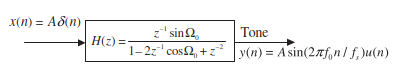
8.11.1 Single‑Tone Digital Generator
We use a second‑order IIR whose impulse response is a sinusoid:
\[
H(z) = \frac{z \sin\Omega_0}{z^2 - 2 z \cos\Omega_0 + 1} = \frac{z^{-1} \sin\Omega_0}{1 - 2 \cos\Omega_0 z^{-1} + z^{-2}}
\]
With sampling rate \(f_s\) and tone frequency \(f_0\) :
\[
\Omega_0 = \frac{2\pi f_0}{f_s}
\]
Difference equation (input \(x(n)\) , output \(y(n)\) ):
\[
y(n) = \sin\Omega_0\,x(n-1) + 2\cos\Omega_0\,y(n-1) - y(n-2)
\]
To generate a pure tone of amplitude A:
Use \(x(n) = A\delta(n)\) (single impulse).
Output \(y(n)\) is the sinusoid.
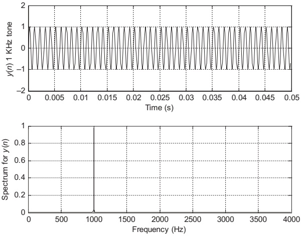
Example: Generate 1 kHz at 8 kHz Sampling
Given: \(f_s = 8000\) Hz, \(f_0 = 1000\) Hz.
Compute:
\[
\Omega_0 = 2\pi\frac{1000}{8000} = \frac{\pi}{4}
\]
\[
\sin\Omega_0 = \sin\left(\frac{\pi}{4}\right) \approx 0.707107
\]
\[
2\cos\Omega_0 = 2\cos\left(\frac{\pi}{4}\right) \approx 1.414214
\]
Filter:
\[
H(z) = \frac{0.707107 z^{-1}}{1 - 1.414214 z^{-1} + z^{-2}}
\]
MATLAB (Program 8.18) uses impulse input to filter this system and plots:
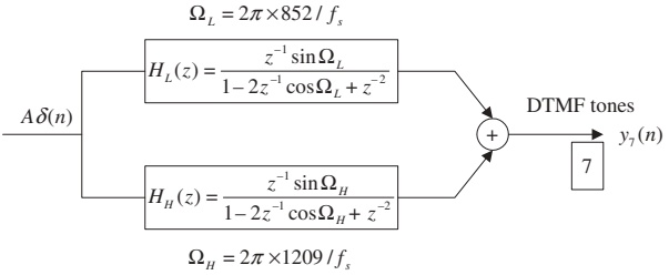
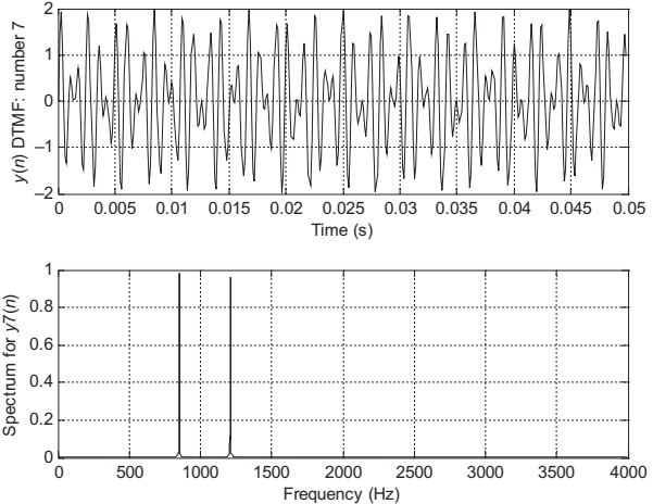
8.11.2 DTMF Dual‑Tone Generator (Key “7”)
To generate key “7”:
Tone 1: 852 Hz
Tone 2: 1209 Hz
Implementation:
Use two second‑order tone generators in parallel.
Sum their outputs.
Program 8.19 (MATLAB) does:
Compute coefficients for 852 Hz and 1209 Hz generating filters.
Filter impulse through each to get y852 and y1209.
Sum: y7 = y852 + y1209.
Result:
8.11.3 Goertzel Algorithm – Motivation
We want to detect specific tones (e.g., only 7 DTMF frequencies) from a signal. Full FFT:
Computes all N DFT bins → unnecessary and heavier.
Goertzel:
Efficiently computes selected DFT coefficients using a second‑order IIR filter .
Especially good for DTMF detection and similar narrowband spectral lines.
Key idea: interpret a DFT bin as the output of a resonator filter excited by the signal.
From DFT to Goertzel – Concept
DFT of length N:
\[
X(k) = \sum_{n=0}^{N-1} x(n) e^{-j\frac{2\pi kn}{N}}
\]
We can rewrite in terms of convolution with a sequence \(h_k(n) = e^{j\frac{2\pi k n}{N}}\) :
\[
X(k) = \sum_{n=0}^{N-1} x(n) h_k(N-n)
\]
If we treat \(h_k(n)\) as an impulse response of an IIR filter:
\[
H_k(z) = \sum_{n=0}^{\infty} h_k(n) z^{-n} = \frac{1}{1 - e^{j\frac{2\pi k}{N}} z^{-1}} = \frac{1}{1 - W_N^{-k} z^{-1}}
\]
After some algebra and multiplying numerator/denominator by \(1 - W_N^k z^{-1}\) :
\[
H_k(z) = \frac{1 - W_N^k z^{-1}}{1 - 2\cos\left(\frac{2\pi k}{N}\right) z^{-1} + z^{-2}}
\]
This is the Goertzel filter – a second‑order resonator with resonance at \(\Omega = 2\pi k/N\) .
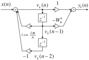
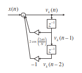
Goertzel Algorithm – Difference Equations
Using direct‑form II (Fig. 8.53):
Algorithm for bin k, length N:
Initialize: \(v_k(-2)=0\) , \(v_k(-1)=0\) .
Append one zero sample: set \(x(N)=0\) .
For \(n = 0, 1, \dots, N\) :
\[
v_k(n) = 2\cos\left(\frac{2\pi k}{N}\right) v_k(n-1) - v_k(n-2) + x(n)
\]
Then:
\[
y_k(n) = v_k(n) - W_N^k\,v_k(n-1)
\]
At n = N:
\[
X(k) = y_k(N)
\]
But in many applications we only need \(|X(k)|\) , not the complex phase.
Magnitude without Complex Arithmetic (Modified Goertzel)
Using the same state sequence \(v_k(n)\) (with \(x(N)=0\) ):
\[
|X(k)|^2 = v_k^2(N) + v_k^2(N-1) - 2\cos\left(\frac{2\pi k}{N}\right) v_k(N) v_k(N-1)
\]
This avoids complex multiplications, only uses real arithmetic.
A simplified filter (Fig. 8.54) has transfer function:
\[
G_k(z) = \frac{V_k(z)}{X(z)} = \frac{1}{1 - 2\cos\left(\frac{2\pi k}{N}\right) z^{-1} + z^{-2}}
\]
Algorithm (modified Goertzel):
Same recurrence for \(v_k(n)\) .
Use formula above to get \(|X(k)|^2\) .
Example 8.26 – Goertzel for X(1) with N=4
Given: \(x(0)=1, x(1)=2, x(2)=3, x(3)=4\) . We want bin \(k=1\) , \(N=4\) .
Compute constants:
\[
2\cos\left(\frac{2\pi}{4}\right) = 0, \quad W_4^1 = e^{-j\frac{\pi}{2}} = -j
\]
Simplified recurrence:
\[
x(4) = 0
\]
For \(n=0,\dots,4\) :
\[
v_1(n) = -v_1(n-2) + x(n)
\]
Output:
\[
y_1(n) = v_1(n) + j v_1(n-1)
\]
Compute sequence step‑by‑step (given in text), final result:
\(X(1) = y_1(4) = -2 + j2\) \(|X(1)|^2 = 8\) Two‑sided amplitude: \(A_1 = \frac{1}{4}\sqrt{8} = 0.7071\)
Single‑sided amplitude: ≈ 1.4141
This matches what you’d get from direct DFT.
Example 8.27 – Modified Goertzel for k=0
Same sequence: \(x = [1,2,3,4]\) , \(k=0\) , \(N=4\) .
Here: \(2\cos(0) = 2\) .
Recurrence:
\[
v_0(n) = 2 v_0(n-1) - v_0(n-2) + x(n)
\]
After computing \(v_0(0)\dots v_0(4)\) :
\(v_0(3) = 20\) , \(v_0(4) = 30\) .
Magnitude:
\[
\begin{aligned}
|X(0)|^2 &= v_0^2(4) + v_0^2(3) - 2 v_0(4)v_0(3) \\
&= 30^2 + 20^2 - 2\cdot30\cdot20 = 100
\end{aligned}
\]
Amplitude:
\[
A_0 = \frac{1}{4}\sqrt{100} = 2.5
\]
Again, matches DFT result.
MATLAB Function – Goertzel Implementation (Program 8.20)
Function interface:
function [Xk , Ak ] = galg (x , k )% x: input vector % k: frequency index % Xk: kth DFT coefficient % Ak: magnitude of kth DFT coefficient (single-sided) Logic:
Let N = length(x), append one zero sample.
Use recurrence to fill array vk.
Compute complex \(X_k\) and magnitude Ak using formula for \(|X(k)|^2\) .
Verification (Example 8.28):
For x = [1 2 3 4], k=1 → X1 ≈ −2 + 2i, A1 ≈ 0.7071.
For x = [1 2 3 4], k=0 → X0 = 10, A0 ≈ 2.5.
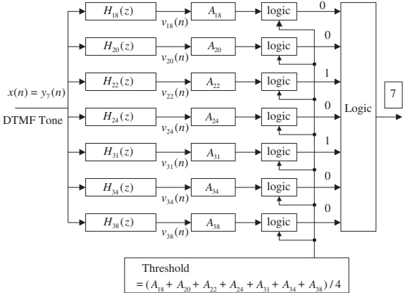
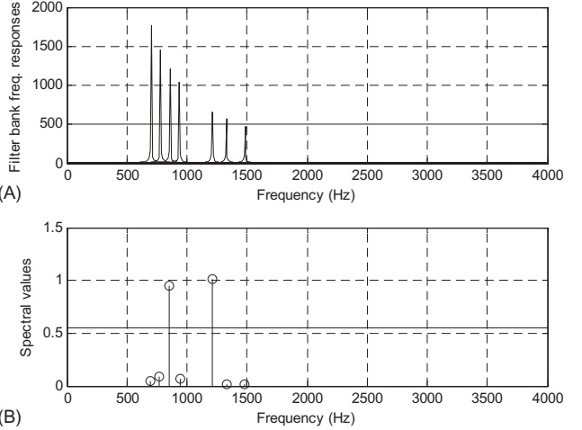
8.11.4 DTMF Detection via Goertzel
For DTMF: we know the 7 possible tone frequencies:
\[
\{697, 770, 852, 941, 1209, 1336, 1477\}\ \text{Hz}
\]
Design:
Choose \(f_s = 8000\) Hz, frame length \(N = 205\) samples.
Map tone frequencies to DFT bin indices by: \[
k = \text{round}\left( \frac{f}{f_s} \cdot N \right)
\]
Table 8.12 (precomputed):
697
18
770
20
852
22
941
24
1209
31
1336
34
1477
38
We implement 7 parallel Goertzel filters , one for each k.
DTMF Detector Block Diagram
Comparison Table – At a Glance
BLT LP, HP, BP, BS
Yes
None
High (but standard)
Impulse Invariant LP, BP (mainly)
Yes (via analog design)
Sampling rate >> cutoff (LP) or >> upper cutoff (BP) to avoid aliasing
Moderate
Pole‑Zero Placement 2nd‑order BP/notch, 1st‑order LP/HP
No (only 3 dB level)
Narrow bands or simple edges; usually low order
Simple
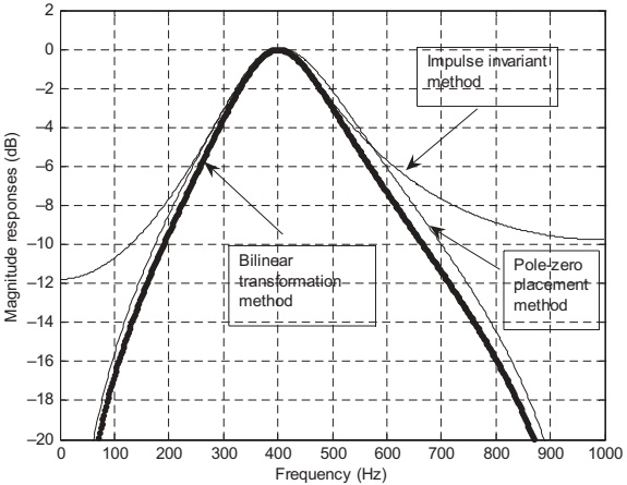
Performance example:
For a bandpass spec: center 400 Hz, BW 200 Hz, fs=2000 Hz, 2nd order Butterworth:
BLT best meets specs.
Pole‑zero placement shows some center frequency shift and wider response if poles not very close to unit circle.
Impulse invariant suffers stopband aliasing unless fs is very high.
Key Takeaways / Summary
IIR filters are powerful for narrowband tasks :
Notch filters → removing line hum and harmonics in ECG.
Bandpass filters → isolating ECG frequencies or communication channels.
Finite precision matters :
Quantized coefficients shift pole/zero locations.
Stability and magnitude response can be impacted – always verify.
Goertzel algorithm :
Efficient when you only need a few DFT bins.
Direct mapping between a target frequency and a second‑order resonator.
Perfectly suited for DTMF detection: small filter bank + logic.
IIR design methods in practice :
Use BLT for most serious filter designs (LP, HP, BP, BS).
Use impulse invariant when you want to mimic analog impulse response and can oversample.
Use pole‑zero placement for quick, simple filters (e.g., small notches, 1st‑order LP/HP), especially in embedded DSP.
General 2nd‑order IIR (biquad):
\[
H(z)=\frac{b_0 + b_1 z^{-1} + b_2 z^{-2}}{1 + a_1 z^{-1} + a_2 z^{-2}}
\]
Difference equation:
\[
y(n) = b_0 x(n) + b_1 x(n-1) + b_2 x(n-2) - a_1 y(n-1) - a_2 y(n-2)
\]
Goertzel recurrence (modified):
State update: \[
v_k(n) = 2\cos\left(\frac{2\pi k}{N}\right) v_k(n-1) - v_k(n-2) + x(n)
\]
Squared magnitude: \[
|X(k)|^2 = v_k^2(N) + v_k^2(N-1) - 2\cos\left(\frac{2\pi k}{N}\right) v_k(N) v_k(N-1)
\]
Single‑sided amplitude: \[
A_k = \frac{2}{N} \sqrt{|X(k)|^2}
\]
Heart‑rate from zero crossings:
\[
HR\ (\text{bpm}) = \frac{60}{N/f_s} \cdot \frac{\text{zero crossings}}{2}
\]
DTMF bin mapping:
\[
k = \text{round}\left( \frac{f}{f_s} N \right)
\]
IIR Filters – Applications & Practical Issues - Interactive Deck
How This Interactive Deck Works
All code runs in your browser using Pyodide (Python compiled to WebAssembly).
You can:
Edit Python code and run it live.
Use interactive sliders (Observable JS) to control parameters.
See Plotly charts update in real time as you adjust the controls.
Tip: Use this deck to experiment with:
60 Hz notch filter behavior.
Goertzel algorithm and DTMF tone detection.
Effects of coefficient changes on poles/zeros.
Explain briefly what Pyodide is and that no separate Python installation is needed. Mention that some cells may take a second to run the first time (Pyodide initialization).
Warm‑Up: Simple Pyodide Code Cell
Try editing the loop range or the formula.
Have students increase the range or change the arithmetic expression. Confirm they see immediate output changes.
1. Exploring a Second‑Order IIR Notch Filter (60 Hz)
Let’s start from the 60 Hz notch filter section used in the ECG hum eliminator.
We’ll implement:
\[
H_1(z) = \frac{0.9803 - 1.5862 z^{-1} + 0.9803 z^{-2}}{1 - 1.5842 z^{-1} + 0.9586 z^{-2}}
\]
and visualize its frequency response .
Ask: where is the notch located? Students should hover around 60 Hz and note the depth. Invite them to change fs or coefficients in the cell to see what happens to the notch.
1.1 Interactive: Move the Notch Frequency
Use the slider to adjust the notch frequency between 40 and 100 Hz and see how the response changes.
= Inputs. range ([40 , 100 ], {step : 2 , label : "Notch center frequency f0 (Hz)" })= Inputs. range ([2 , 10 ], {step : 1 , label : "Approximate 3-dB bandwidth (Hz)" })
Encourage students to increase BW and observe how the notch widens and passband distortion grows. Ask: What happens if BW is very small (poles close to unit circle)? Discuss sensitivity to coefficient quantization.
2. Time‑Domain ECG Notch Filtering (Toy Example)
We’ll create a synthetic ECG‑like pulse plus 60 Hz hum and see how the notch filter cleans it up.
Try: change the hum amplitude or notch frequency and re‑run.
While this is not a fully realistic ECG, it’s enough to show hum removal in time domain. Encourage them to modify hum_amp or add harmonics at 120 Hz, 180 Hz and see remaining oscillation if only one notch is used.
3. Interactive Coefficient Quantization Effect (1st‑Order IIR)
We’ll reproduce the idea from Example 8.24 interactively:
\[
H(z) = \frac{b_0 + b_1 z^{-1}}{1 + a_1 z^{-1}}
\]
Use sliders to adjust the quantized coefficients and watch:
Pole and zero locations.
Magnitude response changes.
= Inputs. range ([0.5 , 1.5 ], {step : 0.01 , label : "b0 (quantized)" })= Inputs. range ([- 0.5 , 0.5 ], {step : 0.01 , label : "b1 (quantized)" })= Inputs. range ([- 0.9 , 0.9 ], {step : 0.01 , label : "a1 (quantized)" })
Ask students to move a1 closer to ±1 and observe the pole on or near the unit circle. Discuss stability: |pole| < 1 is required. This makes the impact of small quantization errors visually clear.
4. Interactive Goertzel Algorithm – Single Bin
We’ll build an interactive Goertzel analyzer for a single DFT bin.
Use sliders to:
Select signal frequency (f_0).
Select DFT bin index k.
Then we’ll compute (|X(k)|) using the modified Goertzel algorithm.
= Inputs. range ([0 , 4000 ], {step : 50 , label : "Signal frequency f0 (Hz)" })= Inputs. range ([0 , 64 ], {step : 1 , label : "DFT bin index k" })
Ask students to choose f0 exactly matching a DFT bin: f0 = k*fs/N, and observe that Goertzel and DFT amplitudes match. Then choose an “off‑bin” frequency and see how energy spreads across bins.
5. DTMF Tone Generation – Try Another Key
Let’s build a small DTMF generator you can experiment with.
We’ll approximate the idea of Program 8.19:
Use the IIR sinusoid generator with impulse input.
Sum two tones for a key.
= Inputs. select ("1" , "2" , "3" , "4" , "5" , "6" , "7" , "8" , "9" , "*" , "0" , "#" , label : "DTMF Key" }
Ask students: verify the two peaks in the spectrum match the standard DTMF frequencies for the chosen key. Next, they can modify fs or T and see effect on frequency resolution.
7. Summary: What to Explore Further
Use these interactive blocks to:
Vary notch filter parameters and see:
How bandwidth and center frequency affect ECG hum rejection.
Change IIR coefficients to understand:
Pole/zero motion vs. stability and magnitude response.
Experiment with the Goertzel algorithm by:
Changing N and k, observing resolution vs. leakage.
Extend the DTMF detector:
Implement a full keypad decoder purely in Python.
Try to break the designs: - What happens if the sampling rate changes but the same coefficients are used? - How sensitive is the DTMF detector to frequency drift or noise?
This kind of hands‑on “stress testing” is a great way to build intuition about real‑world DSP systems.
Encourage students to save interesting parameter combinations and screen captures. Suggest they adapt these snippets for homework, labs, or mini‑projects (e.g., implementing a Goertzel‑based tone detector on a microcontroller).