8.3 Infinite Impulse Response (IIR) Filter Design

Digital Signal Processing

Imron Rosyadi

8.6–8.8 Infinite Impulse Response (IIR) Filter Design and Realization

This entire deck is meant for one or two 50‑minute lectures in an undergraduate DSP course. We’ll move from continuous‑time (analog) filters to discrete‑time (digital) IIR filters, focus on two design approaches (impulse invariant and pole–zero placement), and then show how to implement these filters using direct‑form structures and cascade sections. Emphasize the connection to real ECE systems: audio filters, communication channel filters, and control systems.

Learning Objectives

By the end of this session, you should be able to:

1. Explain the impulse invariant design method and when it is appropriate.
2. Derive a digital IIR transfer function from an analog transfer function using impulse invariance.
3. Describe how pole–zero placement shapes the magnitude response of a digital filter.
4. Design simple IIR filters by manually placing poles and zeros:
   • Second‑order bandpass and bandstop (notch) filters.
   • First‑order lowpass and highpass filters.
5. Implement IIR filters using:
   • Direct‑Form I, Direct‑Form II, and
   • Cascade realization with second‑order sections.

Explicitly map these objectives to exam or project expectations: students will need to derive H(z) from H(s), sketch pole‑zero plots, and write out realization equations or block diagrams. Stress that this chapter also prepares them to interpret what MATLAB’s butter, cheby1, etc., are doing internally.

Real‑World ECE Motivation

Where do IIR filters show up?

• Wireless communications
  • IF bandpass filters, channel shaping
• Audio / speech
  • Equalizers, telephone channel models
• Control systems
  • Digital equivalents of analog compensators
• Sensors & instrumentation
  • Lowpass filters for noise reduction

Why IIR instead of FIR?

• Often achieve sharp transitions with lower order
• Can mimic analog filters (Butterworth, Chebyshev, etc.)

FIG. 8.27 Impulse invariant design concept.

Use a quick analogy: - FIR filters are like “finite memory” systems (moving average). - IIR filters are like analog RC/RLC circuits—feedback gives infinite impulse response and efficient sharp filtering.

Mention that many legacy systems started as analog and were later digitized; impulse invariance is one way to do that translation.

8.6 Impulse Invariant Design: Core Idea

We start with an analog filter:

• Analog transfer function: \(H(s)\)
• Analog impulse response: \(h(t) = \mathcal{L}^{-1}\{H(s)\}\)

Impulse invariant design:

1. Compute analog impulse response \(h(t)\).
2. Sample \(h(t)\) at \(t = nT\) to get \(h(nT)\).
3. Multiply by \(T\) to approximate area: \(T\,h(n) = T\,h(t)\big|_{t=nT}\).
4. Take \(z\)‑transform of \(T\,h(n)\) to obtain \(H(z)\).

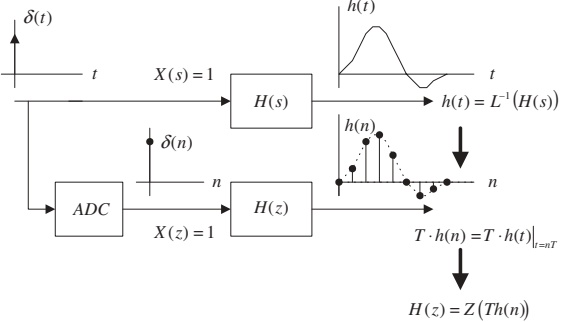
Mathematically:

\[ h(t) = \mathcal{L}^{-1}\{H(s)\} \]

\[ T h(n) = T h(t)\big|_{t=nT},\quad n\ge 0 \]

\[ H(z) = \mathcal{Z}\{T h(n)\} \]

Note

Key idea: The digital impulse response is a sampled (and scaled) version of the analog impulse response. This makes the time‑domain behavior similar, especially for low frequencies.

Emphasize: Unlike the bilinear transform, impulse invariance directly samples the continuous‑time impulse response. Students usually confuse “sample the input” vs “sample the impulse response”; highlight that here we are sampling \(h(t)\) itself. We scale by \(T\) because the integral (area) of the analog impulse response should match the sum (area of rectangles) of the digital impulse response.

Area and DC Gain Matching

The scaling factor \(T\) is chosen so that the area under \(h(t)\) matches the sum of \(T h(n)\):

\[ \int_0^{\infty} h(t)\,dt \;\approx\; T h(0) + T h(1) + T h(2) + \cdots \]

• Left side: DC gain of the analog filter.
• Right side: DC gain of the digital filter.

As \(T \to 0\) (sampling frequency \(f_s = 1/T \to \infty\)):

• Rectangular approximation becomes very accurate.
• DC gain of digital filter \(\approx\) DC gain of analog filter.

But for practical \(T\), we may need extra gain scaling to match an exact DC gain.

Connect this to Riemann sums from calculus: the sum \(T\sum h(n)\) approximates the integral. Point out that in Example 8.15, they later rescale \(H(z)\) to enforce unit DC gain, which is common practice when the passband gain is specified.

Example 8.15 – Analog to Digital (1/3)

Given analog transfer function:

\[ H(s) = \frac{2}{s + 2} \]

Sampling rate: \(f_s = 10\ \text{Hz} \Rightarrow T = 0.1\ \text{s}\)

Step 1: Inverse Laplace transform to get analog impulse response:

\[ h(t) = \mathcal{L}^{-1}\left\{\frac{2}{s + 2}\right\} = 2 e^{-2t} u(t) \]

Step 2: Sample and scale:

\[ T h(n) = T \cdot 2 e^{-2nT} u(n) = 0.2 e^{-0.2 n} u(n) \]

Step 3: Use \(z\)‑transform pair (Chapter 5):

\[ \mathcal{Z}\{e^{-a n} u(n)\} = \frac{z}{z - e^{-a}} \]

Here, \(a = 0.2\), so \(e^{-a} = e^{-0.2} \approx 0.8187\).

Clarify \(a\): The discrete‑time sequence is \(e^{-a n}\) with \(a>0\). Here \(e^{-a} = e^{-0.2}\) is the common ratio of the exponential sequence. Also remind students that \(u(n)\) (unit step) ensures causality (\(n \ge 0\)).

Example 8.15 – Analog to Digital (2/3)

Apply the \(z\)‑transform to \(T h(n)\):

\[ H(z) = \mathcal{Z}\{0.2 e^{-0.2n} u(n)\} = 0.2 \,\mathcal{Z}\{e^{-0.2n} u(n)\} = 0.2\,\frac{z}{z - 0.8187} \]

Express in standard IIR form:

\[ H(z) = \frac{0.2 z}{z - 0.8187} = \frac{0.2}{1 - 0.8187 z^{-1}} \]

This is a first‑order IIR lowpass‑like filter with:

• One pole at \(z = 0.8187\) (inside unit circle)
• One zero at \(z = 0\)

Tip

To quickly sketch the frequency response: - Pole close to \(z=1\) → large low‑frequency gain - Zero at \(z=0\) → attenuates high frequencies.

Show or sketch a simple pole–zero plot on the board: - Real axis: mark 0.8187; that’s the pole. - Zero at origin. Use this to intuitively justify why the magnitude response looks lowpass. Mention that the exact magnitude and phase responses are plotted in MATLAB (Program 8.12).

Example 8.15 – Frequency Response (3/3)

MATLAB (Program 8.12) computes:

1. Analog frequency response \(H(j\omega)\) using freqs.
2. Digital frequency response \(H(e^{j\Omega})\) using freqz.

Main observations (Fig. 8.28):

• The magnitude responses of analog and digital filters closely match in shape for \(f\) below about \(1.8\ \text{Hz}\).

• There is a DC gain mismatch:

  \[ H(e^{j\Omega})\big|_{\Omega=0} = H(1) = 1.1031 \]

To enforce unit DC gain, scale \(H(z)\):

\[ H(z) = \frac{1}{1.1031}\,\frac{0.2}{1 - 0.8187 z^{-1}} = \frac{0.1813}{1 - 0.8187 z^{-1}} \]

Middle plot of Fig. 8.28 shows the scaled magnitude response, now matching the analog much better in passband.

Point out how gain scaling is routinely done in filter design: - Design the basic structure for the right shape. - Then scale gain to match specifications (e.g., unit DC gain, 0 dB at center frequency).

Encourage students to run Program 8.12 and modify T (sampling interval) to see the effect on aliasing visually.

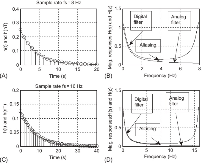
Aliasing in Impulse Invariant Design

Key issue: The analog impulse response \(h(t)\) is generally not band‑limited.

Sampling \(h(t)\) at rate \(f_s\):

• Any frequency content above Nyquist frequency \(f_s/2\) gets aliased back into \([0, f_s/2]\).
• This causes distortion in the digital filter’s frequency response.

Fig. 8.29 shows this numerically for Example 8.15:

• (A, B): Sampling at \(f_s = 8\ \text{Hz}\) (T=0.125 s) → strong aliasing, poor match.
• (C, D): Sampling at \(f_s = 16\ \text{Hz}\) → less aliasing, better magnitude match.

FIG. 8.29

Warning

Aliasing cannot be eliminated in the impulse invariant method because we sample a non‑band‑limited impulse response. We can only reduce aliasing by: - Increasing sampling frequency \(f_s\), or - Designing the analog filter with a very low cutoff frequency.

Use a real‑world analogy: sampling a sharp spike vs sampling a smooth sine wave. Sharp, fast decay in time often implies high‑frequency content in frequency domain.

Stress that this is why the impulse invariant method is not recommended for highpass or bandstop filters: those responses inherently concentrate energy near the folding frequency, where aliasing is worst.

When to Use Impulse Invariance

From the aliasing analysis:

• Analog highpass or bandstop filters have significant energy near the Nyquist limit even when oversampled.
• Sampling their impulse responses leads to maximum aliasing.

So:

• Do not use impulse invariance alone to design digital highpass or bandstop IIR filters (unless using extra anti‑aliasing or prewarping tricks).
• Prefer bilinear transform (BLT) for highpass or bandstop designs.

Impulse invariant design is appropriate for:

• Lowpass filters.
• Bandpass filters when sampling rate is much larger than the largest passband frequency.

Important

Rule of thumb: Use impulse invariant for low frequency, lowpass/bandpass designs with high oversampling. Use BLT for highpass / bandstop and more general cases.

Tie this back to design flow: - If the analog prototype is already given (e.g., from a control engineer), choose the digital mapping. - If you must preserve time‑domain shape (e.g., step responses), impulse invariance can be attractive, but always check aliasing.

Example 8.16 – Second‑Order Bandpass via Impulse Invariance (1/3)

Given analog transfer function:

\[ H(s) = \frac{s}{s^2 + 2s + 5} \]

Sampling rate: \(f_s = 10\ \text{Hz} \Rightarrow T = 0.1\ \text{s}\)

Step 1: Complete the square in denominator:

\[ H(s) = \frac{s}{(s+1)^2 + 2^2} \]

Rewrite numerator to match table form:

\[ H(s) = \frac{(s+1) - 1}{(s+1)^2 + 2^2} = \frac{s+1}{(s+1)^2 + 2^2} - 0.5\frac{2}{(s+1)^2 + 2^2} \]

Use Laplace transform table:

• \(\mathcal{L}^{-1}\big\{\frac{s+a}{(s+a)^2 + \omega_0^2}\big\} = e^{-a t}\cos(\omega_0 t) u(t)\)
• \(\mathcal{L}^{-1}\big\{\frac{\omega_0}{(s+a)^2 + \omega_0^2}\big\} = e^{-a t}\sin(\omega_0 t) u(t)\)

So analog impulse response is:

\[ h(t) = e^{-t}\cos(2t)\,u(t) - 0.5 e^{-t}\sin(2t)\,u(t) \]

Highlight that this is a typical underdamped second‑order system: exponentially decaying sinusoid. Students should recognize that such systems often correspond to bandpass behavior. The two terms correspond to cosine and sine components.

Example 8.16 – Sampling and \(z\)‑Transform (2/3)

Sample and scale: \(T=0.1\)

\[ \begin{aligned} T h(n) &= T h(t)\big|_{t=nT} \\ &= 0.1 e^{-0.1n}\cos(0.2n) u(n) \\ &\quad - 0.05 e^{-0.1n}\sin(0.2n) u(n) \end{aligned} \]

Apply \(z\)‑transform (using formulas from Chapter 5):

\[ \begin{aligned} H(z) &= \mathcal{Z}\left\{0.1 e^{-0.1n}\cos(0.2n) u(n)\right\} \\ &\quad - \mathcal{Z}\left\{0.05 e^{-0.1n}\sin(0.2n) u(n)\right\} \\ &= \frac{0.1z(z - e^{-0.1}\cos(0.2))}{z^2 - 2 e^{-0.1}\cos(0.2) z + e^{-0.2}} \\ &\quad - \frac{0.05 e^{-0.1}\sin(0.2) z}{z^2 - 2 e^{-0.1}\cos(0.2) z + e^{-0.2}} \end{aligned} \]

After algebraic simplification, we obtain:

\[ H(z) = \frac{0.1 - 0.09767 z^{-1}}{1 - 1.7735 z^{-1} + 0.8187 z^{-2}} \]

Emphasize that the denominator corresponds to a pair of complex conjugate poles, consistent with the analog poles at \(s=-1 \pm 2j\). The digital poles are inside the unit circle, and the real parts relate to the discrete damping factor \(e^{-0.1}\). Encourage students to verify the coefficients using MATLAB’s symbolic toolbox (or Python) as a quick check.

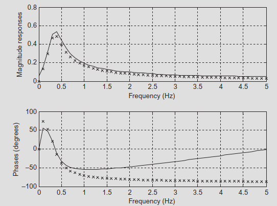
Example 8.16 – Frequency Response (3/3)

Program 8.13 uses:

• freqs([10],[1 2 5],w) (conceptually) for the analog \(H(s)\)
• freqz([0.1 -0.09766],[1 -1.7735 0.8187], length(w)) for the digital \(H(z)\)

FIG. 8.30

Observations:

• The shape of the digital filter’s magnitude response (bandpass) matches the analog filter’s shape.
• The passband gain is higher for the digital filter; again, gain scaling can be applied if unit gain is required.

Tip

When comparing analog and digital designs: - Match frequency axes in Hz: use \(\Omega = 2\pi f T\) for digital. - Focus on shape (location of peaks, nulls, bandwidth) first, then adjust gain.

This is a good place to ask students: - Where do you expect the center frequency to be in Hz? - How does the sampling rate relate to the discrete‑time frequency where the peak occurs?

Also note that impulse invariance preserves the analog impulse response shape at integer multiples of \(T\), which often indirectly preserves resonant frequencies reasonably well for sufficiently large \(f_s\).

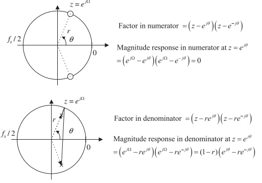
8.7 Pole–Zero Placement: Intuition

In the \(z\)‑plane, consider placing poles and zeros and evaluating the response on the unit circle \(z = e^{j\Omega}\).

• Place a zero at angle \(\theta\) on the unit circle: \(z_0 = e^{j\theta}\).
  • Numerator factor: \((z - e^{j\theta})(z - e^{-j\theta})\).
  • At \(\Omega = \theta\), one factor is \((e^{j\theta} - e^{j\theta}) = 0\) → magnitude null.
• Place poles at \(z_p = r e^{\pm j\theta}\), with \(r < 1\):
  • Denominator factor: \((z - re^{j\theta})(z - re^{-j\theta})\).
  • At \(\Omega = \theta\), distance from \(e^{j\theta}\) to pole is \((1 - r)\) → small denominator → large magnitude.

FIG. 8.31

Note

Rule of thumb:

• Zeros suppress magnitude near their angle.
• Poles boost magnitude near their angle.

Draw a quick sketch: - Unit circle. - A zero on the circle and a pole just inside, both at the same angle. Then trace how distances from evaluation point \(e^{j\Omega}\) change as \(\Omega\) sweeps around the circle.

This geometric view is extremely powerful and will be reused when designing bandpass, bandstop, lowpass, and highpass filters by hand.

Application of Pole–Zero Placement

By combining pole and zero placements, we can create different filter types:

• Lowpass:
  • Pole(s) near \(z=1\), zeros near \(z=-1\) or on unit circle at higher frequencies.
• Highpass:
  • Zero at \(z=1\) (kill DC), pole closer to \(z=-1\) to emphasize high frequencies.
• Bandpass:
  • Complex poles at angle \(\theta_0\) (center frequency); zeros at DC and Nyquist to attenuate outside band.
• Bandstop (notch):
  • Zeros on the unit circle at \(\theta_0\) (notch frequency); poles near zeros (inside unit circle) to restore neighboring frequencies.

Pole–zero placement is:

• Intuitive and approximate.
• Very useful for simple filters with narrow bands or extreme cutoff frequencies.

Stress that this is not the same as systematic design (Butterworth, Chebyshev) but is excellent for quick designs and for understanding how pole locations affect response. In many embedded systems, simple pole–zero designs are enough and easier to implement and tune by hand.

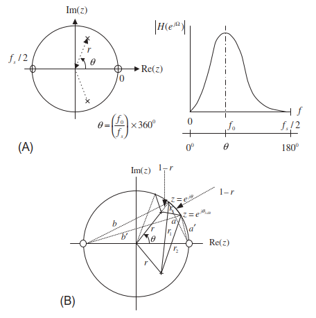
8.7.1 Second‑Order Bandpass Filter – Geometry

Typical placement for a narrow bandpass (Fig. 8.32A):

• Complex poles: \(z = r e^{\pm j\theta}\)
  • Radius \(r\) controls bandwidth.
  • Angle \(\theta\) sets center frequency.
• Zeros: at \(z = 1\) and \(z = -1\)
  • Zero gain at DC and folding frequency \(f_s/2\).

FIG. 8.32

Center frequency angle:

\[ \theta = \left(\frac{f_0}{f_s}\right) \times 360^\circ \]

Bandwidth (approximate narrowband formula):

\[ r \approx 1 - \pi\frac{BW_{3\text{dB}}}{f_s},\quad 0.9 \le r < 1 \]

Explain the derivation idea: - At center frequency, poles are very close to unit circle → large gain. - At 3 dB points, geometry yields \(r_3 = \sqrt{2(1 - r)}\) and then bandwidth \(\approx 2(1-r)\) in normalized radian frequency, leading to \(r = 1 - \pi BW_{3dB} / f_s\).

Students don’t need to memorize the geometric derivation; they should remember the design formulas and the interpretation.

Second‑Order Bandpass Filter – Transfer Function

General transfer function:

\[ H(z) = \frac{K (z - 1)(z + 1)}{(z - r e^{j\theta})(z - r e^{-j\theta})} = \frac{K(z^2 - 1)}{z^2 - 2 r \cos\theta\, z + r^2} \]

Design formulas summary:

• Center frequency:

  \[ \theta = \left(\frac{f_0}{f_s}\right) 360^\circ \]

• Pole radius:

  \[ r \approx 1 - \pi \frac{BW_{3\text{dB}}}{f_s},\quad 0.9 \le r < 1 \]

• Gain scaling for unit passband gain:

  \[ K = \frac{(1 - r)\sqrt{1 - 2 r \cos(2\theta) + r^2}}{2|\sin\theta|} \]

Tip

Implementation form (for code):

\[ H(z) = \frac{b_0 + b_2 z^{-2}}{1 - a_1 z^{-1} + a_2 z^{-2}} \]

where \(b_0 = K\), \(b_1 = 0\), \(b_2 = -K\), \(a_1 = 2 r \cos\theta\), \(a_2 = -r^2\) (after factoring a \(z^2\) in numerator and denominator).

Clarify: we can write the denominator as \(z^2 - 2r\cos\theta z + r^2 = z^2 (1 - 2r\cos\theta z^{-1} + r^2 z^{-2})\) and then read off the IIR coefficients. Students will frequently convert between polynomial in \(z\) (for math) and polynomial in \(z^{-1}\) (for implementation).

Example 8.17 – Second‑Order Bandpass Design

Specifications:

• Sampling rate: \(f_s = 8000\ \text{Hz}\)
• Center frequency: \(f_0 = 1000\ \text{Hz}\)
• 3‑dB bandwidth: \(BW = 200\ \text{Hz}\)
• Zero gain at 0 Hz and 4000 Hz (DC and Nyquist)

Step 1: Compute pole radius \(r\):

\[ r = 1 - \pi \frac{BW}{f_s} = 1 - \pi \frac{200}{8000} = 0.9215 \]

Step 2: Center frequency angle:

\[ \theta = \frac{f_0}{f_s} 360^\circ = \frac{1000}{8000} 360^\circ = 45^\circ \]

Step 3: Gain factor \(K\):

\[ K = \frac{(1 - 0.9215)\sqrt{1 - 2(0.9215)\cos(90^\circ) + 0.9215^2}}{2|\sin 45^\circ|} = 0.0755 \]

Final transfer function:

\[ H(z) = \frac{0.0755(z^2 - 1)}{z^2 - 2(0.9215)\cos 45^\circ z + 0.9215^2} = \frac{0.0755 - 0.0755 z^{-2}}{1 - 1.3031 z^{-1} + 0.8491 z^{-2}} \]

Ask: What is the qualitative shape of this filter? - A narrow bandpass centered at 1000 Hz, strong rejection at DC and 4000 Hz.

You can show how to plug this into MATLAB:

b = [0.0755 0 -0.0755];
a = [1 -1.3031 0.8491];
freqz(b,a,1024,8000);

and observe the magnitude plot.

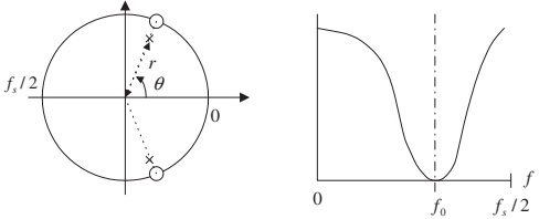
8.7.2 Second‑Order Bandstop (Notch) Filter – Geometry

For a notch (or bandstop) filter:

• Poles: same as bandpass, \(z = r e^{\pm j\theta}\).
• Zeros: placed on the unit circle at \(z = e^{\pm j\theta}\) (the notch frequency).

FIG. 8.33

Design formulas:

• Center (notch) frequency:

  \[ \theta = \left(\frac{f_0}{f_s}\right) 360^\circ \]

• Pole radius:

  \[ r \approx 1 - \pi \frac{BW_{3\text{dB}}}{f_s},\quad 0.9 \le r < 1 \]

Transfer function:

\[ H(z) = \frac{K (z - e^{j\theta})(z - e^{-j\theta})}{(z - r e^{j\theta})(z - r e^{-j\theta})} = \frac{K(z^2 - 2 z\cos\theta + 1)}{z^2 - 2 r z\cos\theta + r^2} \]

Unit passband gain factor:

\[ K = \frac{1 - 2r\cos\theta + r^2}{2 - 2\cos\theta} \]

Explain why zeros at \(e^{\pm j\theta}\) notch out that frequency: at \(z=e^{j\theta}\) the numerator is zero, so \(|H(e^{j\theta})| = 0\). The nearby poles (inside) ensure that frequencies around the notch are not overly attenuated, leading to a narrow notch.

Typical application: removing 50/60 Hz mains hum from biomedical or audio signals.

Example 8.18 – Notch Filter Design

Specifications:

• Sampling rate: \(f_s = 8000\ \text{Hz}\)
• Center (notch) frequency: \(f_0 = 1500\ \text{Hz}\)
• 3‑dB bandwidth: \(BW = 100\ \text{Hz}\)

Step 1: Pole radius:

\[ r \approx 1 - \pi\frac{100}{8000} = 0.9607 \]

Step 2: Angle \(\theta\):

\[ \theta = \frac{1500}{8000} 360^\circ = 67.5^\circ \]

Step 3: Gain factor \(K\):

\[ K = \frac{1 - 2(0.9607)\cos 67.5^\circ + 0.9607^2}{2 - 2\cos 67.5^\circ} = 0.9620 \]

Final transfer function:

\[ H(z) = \frac{0.9620(z^2 - 2 z\cos 67.5^\circ + 1)} {z^2 - 2(0.9607) z\cos 67.5^\circ + 0.9607^2} \]

\[ = \frac{0.9620 - 0.7363 z^{-1} + 0.9620 z^{-2}} {1 - 0.7353 z^{-1} + 0.9229 z^{-2}} \]

Note: there is a small discrepancy in the last denominator coefficient in the text (should be + 0.9229 z^{-2} after normalization w.r.t. \(z^2\)). Encourage students to verify the entire design in MATLAB with freqz and visually confirm the deep notch at 1500 Hz.

You can also show how slight changes in \(r\) affect the notch width.

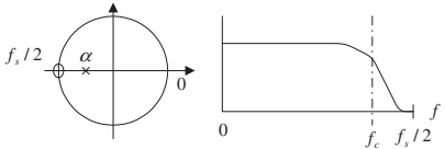
8.7.3 First‑Order Lowpass Filter – Case 1: \(f_c < f_s/4\)

Pole–zero placement (Fig. 8.34A):

• One real pole at \(z = \alpha\) on real axis.
• One zero at \(z = -1\) to force zero gain at Nyquist \(f_s/2\).

FIG. 8.34

Approximate derivation:

• DC magnitude:

  \[ \left|H(e^{j0})\right| = \frac{\text{dist from }1 \text{ to } -1}{\text{dist from }1 \text{ to }\alpha} = \frac{2}{1 - \alpha} \]

• At 3‑dB cutoff, approximate distance geometry leads to:

  \[ 2\pi f_c T = 1 - \alpha \]

Therefore, pole location:

\[ \alpha = 1 - 2\pi \frac{f_c}{f_s} \]

Valid when \(f_c < f_s/4\) and \(\alpha \approx 0.9\,\text{to}\,1\).

Important

Design formulas – Lowpass (case 1):

• If \(f_c < f_s/4\):

  \[ \alpha \approx 1 - 2\pi\frac{f_c}{f_s},\quad 0.9 \le \alpha < 1 \]

• Transfer function:

  \[ H(z) = \frac{K (z + 1)}{z - \alpha},\quad K = \frac{1 - \alpha}{2} \]

Geometric view: - At DC, distance to zero (\(-1\)) is 2; at the pole, it is \(1-\alpha\). - At \(f_c\), the magnitude is down by \(1/\sqrt{2}\) relative to DC.

This is an approximate design, good enough for simple smoothing filters or control loop filters.

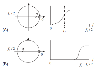
First‑Order Lowpass – Case 2: \(f_c > f_s/4\)

When the cutoff frequency is above \(f_s/4\), we reposition the pole near \(z = -1\) (Fig. 8.35).

FIG. 8.35

Approximate design formula:

• For \(f_c > f_s/4\):

  \[ \alpha \approx -\big(1 - \pi + 2\pi\frac{f_c}{f_s}\big),\quad -1 < \alpha \le -0.9 \]

Transfer function is still:

\[ H(z) = \frac{K(z + 1)}{z - \alpha},\quad K = \frac{1 - \alpha}{2} \]

Intuition: we want the passband to extend closer to Nyquist, so the pole moves closer to \(z = -1\), and the zero at \(-1\) now plays a different role. This is less common in practice; often designers will switch to a more systematic IIR design or use a different sampling rate. But this formula is useful if you are heavily constrained and need a simple 1st‑order design.

Example 8.19 – First‑Order Lowpass

Specifications:

• Sampling rate: \(f_s = 8000\ \text{Hz}\)
• 3‑dB cutoff frequency: \(f_c = 100\ \text{Hz}\)
• Zero gain at 4000 Hz (Nyquist)

Since \(f_c = 100\ \text{Hz} \ll f_s/4 = 2000\ \text{Hz}\), use case 1 formula:

\[ \alpha \approx 1 - 2\pi\frac{100}{8000} = 0.9215 \]

Scale factor:

\[ K = \frac{1 - \alpha}{2} = \frac{1 - 0.9215}{2} = 0.03925 \]

Transfer function:

\[ H(z) = \frac{0.03925(z + 1)}{z - 0.9215} = \frac{0.03925 + 0.03925 z^{-1}}{1 - 0.9215 z^{-1}} \]

Alternative way to compute \(K\):

• DC gain of unscaled filter:

  \[ \text{DC gain} = \frac{z+1}{z-0.9215}\Bigg|_{z=1} = \frac{2}{1 - 0.9215} = 25.4777 \]

• Set \(K = 1 / 25.4777 = 0.03925\).

Highlight that verifying gain via \(H(1)\) is a very general trick for lowpass filters. Ask students which property of the filter response the numerator \((z+1)\) is enforcing (zero at Nyquist).

Also show how to derive the time‑domain recursion: \(y(n) = -0.9215 y(n-1) + 0.03925 x(n) + 0.03925 x(n-1)\).

8.7.4 First‑Order Highpass Filter

Very similar structure, but we swap the location of the zero:

• Zero at \(z = 1\) → kills DC.
• Pole at \(z = \alpha\) on real axis.

Two cases again:

• If \(f_c < f_s/4\), then \(\alpha \approx 1 - 2\pi\frac{f_c}{f_s}\), \(0.9 \le \alpha < 1\).
• If \(f_c > f_s/4\), then \(\alpha \approx -\left(1 - \pi + 2\pi \frac{f_c}{f_s}\right)\), \(-1 < \alpha \le -0.9\).

Transfer function:

\[ H(z) = \frac{K(z - 1)}{z - \alpha},\quad K = \frac{1 + \alpha}{2} \]

FIG. 8.36

Note

Compare with lowpass:

• Lowpass: zero at \(z=-1\), numerator \((z+1)\).
• Highpass: zero at \(z=1\), numerator \((z-1)\).

Remind students that \(z=1\) on the unit circle corresponds to \(\Omega = 0\) (DC), and \(z=-1\) corresponds to \(\Omega = \pi\) (Nyquist). Thus, by choosing where to place zeros, we can control which extreme of the spectrum is attenuated.

Example 8.20 – First‑Order Highpass

Specifications:

• Sampling rate: \(f_s = 8000\ \text{Hz}\)
• 3‑dB cutoff frequency: \(f_c = 3800\ \text{Hz}\)
• Zero gain at 0 Hz (DC)

Since \(f_c = 3800\ \text{Hz} > f_s/4 = 2000\ \text{Hz}\), use highpass case 2 formula:

\[ \alpha \approx -\left(1 - \pi + 2\pi\frac{3800}{8000}\right) = -0.8429 \]

Scale factor (note: the text appears to have a minor sign typo):

The correct highpass formula is typically:

\[ K = \frac{1 + \alpha}{2} = \frac{1 - 0.8429}{2} = 0.07855\ (\text{approx}) \]

Transfer function:

\[ H(z) = \frac{0.07854(z - 1)}{z + 0.8429} = \frac{0.07854 - 0.07854 z^{-1}}{1 + 0.8429 z^{-1}} \]

Alternative: enforce unity gain at Nyquist (\(z = -1\)):

• Passband gain:

  \[ \frac{z - 1}{z + 0.8429}\Bigg|_{z=-1} = \frac{-1 - 1}{-1 + 0.8429} = 12.7307 \]

• So \(K = 1 / 12.7307 = 0.07854\).

Ask students: - How does this differ from the lowpass example structurally? - What is the time‑domain recursion?

\(y(n) = -0.8429 y(n-1) + 0.07854 x(n) - 0.07854 x(n-1)\).

Also, connect this to applications like DC blocking in audio or biomedical signals.

8.8 Realization Structures for IIR Filters

Once we have the transfer function \(H(z)\), we need to implement it in hardware or software.

Common realization forms:

1. Direct‑Form I
2. Direct‑Form II
3. Cascade form using second‑order sections

Trade‑offs:

• Memory usage (# of delay elements)
• Numerical stability and sensitivity to coefficient quantization
• Ease of mapping into code or DSP instructions

Tip

In practice, engineers often: - Factor a high‑order design into biquad (2nd‑order) sections. - Implement each biquad in direct‑form II transposed (for good numerical properties).

Remind students of Chapter 6 FIR realizations: direct forms carry over here but now we have feedback as well as feedforward paths. The presence of feedback means we must be more careful with numerical effects and stability.

Example 8.21 – Direct‑Form I Realization (1/2)

Given first‑order highpass Butterworth filter:

\[ H(z) = \frac{0.1936 - 0.1936 z^{-1}}{1 + 0.6128 z^{-1}} \]

Identify coefficients:

• Numerator: \(b_0 = 0.1936,\ b_1 = -0.1936\)
• Denominator: \(a_0 = 1,\ a_1 = 0.6128\)

Difference equation (from \(H(z)\)):

\[ y(n) = -0.6128 y(n-1) + 0.1936 x(n) - 0.1936 x(n-1) \]

Direct‑Form I structure (Fig. 8.37):

FIG. 8.37

Explain that Direct‑Form I uses two parallel paths: - FIR part (feedforward) using \(b_k\) coefficients. - IIR part (feedback) using \(a_k\) coefficients.

The structure directly mirrors the difference equation. Make sure students can sketch this from the difference equation without looking at the figure.

Example 8.21 – MATLAB Implementation (2/2)

Program 8.14 implements Direct‑Form I manually:

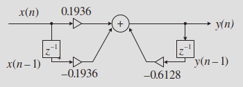
sample = 2:2:20;      % Input test array
x = [0 0];            % Input buffer [x(n) x(n-1)]
y = [0 0];            % Output buffer [y(n) y(n-1)]
b = [0.1936 -0.1936]; % Numerator coefficients
a = [1 0.6128];       % Denominator coefficients

for n = 1:1:length(sample)
    % Shift buffers
    for k = 2:-1:2
        x(k) = x(k-1);
        y(k) = y(k-1);
    end
    x(1) = sample(n);
    y(1) = 0; % Initialize output

    % FIR (feedforward) part
    for k = 1:1:2
        y(1) = y(1) + x(k)*b(k);
    end

    % IIR (feedback) part
    for k = 2:2
        y(1) = y(1) - a(k)*y(k);
    end

    out(n) = y(1);
end
out

Note

In practice, you rarely write this loop manually. You use:

out = filter(b, a, sample);

This code is mainly pedagogical, showing how the delay buffers implement the recursion. It’s a good exercise to trace the first few iterations by hand to verify that the code matches the difference equation. Also stress that a(1) is assumed to be 1 (normalized).

Example 8.22 – Direct‑Form II Realization (1/2)

Given second‑order filter:

\[ H(z) = \frac{0.7157 + 1.4314 z^{-1} + 0.7157 z^{-2}} {1 + 1.3490 z^{-1} + 0.5140 z^{-2}} \]

Coefficients:

• \(b_0 = 0.7157,\ b_1 = 1.4314,\ b_2 = 0.7157\)
• \(a_0 = 1,\ a_1 = 1.3490,\ a_2 = 0.5140\)

Direct‑Form II uses an internal state \(w(n)\):

\[ \begin{aligned} w(n) &= x(n) - a_1 w(n-1) - a_2 w(n-2) \\ y(n) &= b_0 w(n) + b_1 w(n-1) + b_2 w(n-2) \end{aligned} \]

Fig. 8.38 shows the Direct‑Form II block diagram.

FIG. 8.38

Tip

Direct‑Form II reuses the same delay line for feedforward and feedback, which halves the number of delay elements compared to Direct‑Form I.

Explain the concept of the canonical form: minimal number of memory elements. However, in finite‑word‑length systems, Direct‑Form II can be more sensitive to coefficient quantization; often DF‑II transposed is used in practice.

Example 8.22 – MATLAB Implementation (2/2)

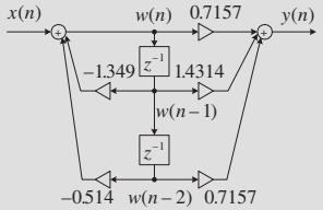
Program 8.15 manually implements Direct‑Form II:

sample = 2:2:20;                 % Input test array
x = [0];                         % Input buffer [x(n)]
y = [0];                         % Output buffer [y(n)]
w = [0 0 0];                     % Internal states [w(n) w(n-1) w(n-2)]
b = [0.7157 1.4314 0.7157];      % Numerator coefficients
a = [1 1.3490 0.5140];           % Denominator coefficients

for n = 1:1:length(sample)
    % Shift w(n) states
    for k = 3:-1:2
        w(k) = w(k-1);
    end
    x(1) = sample(n);

    % IIR (feedback) stage: compute w(n)
    w(1) = x(1);
    for k = 2:1:3
        w(1) = w(1) - a(k)*w(k);
    end

    % FIR (feedforward) stage: compute y(n)
    y(1) = 0;
    for k = 1:1:3
        y(1) = y(1) + b(k)*w(k);
    end

    out(n) = y(1);
end
out

Again, this is equivalent to:

out = filter(b, a, sample);

Highlight that here \(w(n)\) is the state vector of the filter, and this structure maps well to hardware implementations. Ask students which form (direct I vs direct II) is more memory‑efficient and which might be more numerically robust.

This sets up the next topic: cascade realizations, which use multiple biquads.

8.8.2 Cascade Form for Higher‑Order IIR Filters (1/2)

High‑order IIR filters are typically factored into second‑order sections:

\[ H(z) = H_1(z)\, H_2(z)\,\cdots H_M(z) \]

Each \(H_k(z)\) is a second‑order (biquad) filter implemented via Direct‑Form I or II.

Example 8.23:

Given 4th‑order filter:

\[ H(z) = \frac{0.5108z^{2}+1.0215z+0.5108}{z^{2}+0.5654z+0.4776} \times \frac{0.3730z^{2}+0.7460z+0.3730}{z^{2}+0.4129z+0.0790} \]

Write each as standard second‑order section in \(z^{-1}\):

\[ H_1(z) = \frac{0.5108 + 1.0215 z^{-1} + 0.5108 z^{-2}} {1 + 0.5654 z^{-1} + 0.4776 z^{-2}} \]

\[ H_2(z) = \frac{0.3730 + 0.7460 z^{-1} + 0.3730 z^{-2}} {1 + 0.4129 z^{-1} + 0.0790 z^{-2}} \]

The advantage: each biquad is easier to implement and tune, and the cascade form is more numerically stable (less sensitive to coefficient quantization and scaling). DSP libraries like MATLAB’s sosfilt work with these second‑order sections.

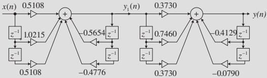
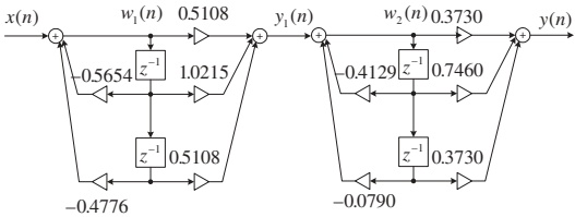
Example 8.23 – Cascade Realization (2/2)

Direct‑Form I cascade (Fig. 8.39):

FIG. 8.39

Difference equations – first section:

\[ \begin{aligned} y_1(n) &= -0.5654 y_1(n-1) - 0.4776 y_1(n-2) \\ &\quad + 0.5108 x(n) + 1.0215 x(n-1) + 0.5108 x(n-2) \end{aligned} \]

Second section:

\[ \begin{aligned} y(n) &= -0.4129 y(n-1) - 0.0790 y(n-2) \\ &\quad + 0.3730 y_1(n) + 0.7460 y_1(n-1) + 0.3730 y_1(n-2) \end{aligned} \]

Direct‑Form II cascade (Fig. 8.40) just replaces each second‑order block with its DF‑II implementation:

FIG. 8.40

In both cases, output of section 1 (\(y_1(n)\) or \(w_1\) outputs) becomes input to section 2.

Connect this to real practice: - MATLAB’s tf2sos or zp2sos functions factor a high‑order filter into second‑order sections. - Good implementations then apply section scaling and use DF‑II transposed for each biquad.

Ask students why we prefer multiple 2nd‑order sections rather than one giant 4th‑order section: - Numerical stability, easier debugging, modular design.

Summary / Key Points

1. Impulse invariant design:
   • Sample and scale the analog impulse response \(h(t)\) to obtain digital \(h[n]\).
   • Works well for lowpass and bandpass with high sampling rates.
   • Suffers from aliasing because \(h(t)\) is not band‑limited.
2. Pole–zero placement:
   • Geometric design of simple IIRs using intuition about how poles/zeros shape the response.
   • Second‑order bandpass and bandstop (notch) filters: complex poles with radius \(r\) and angle \(\theta\).
   • First‑order lowpass and highpass: real pole \(\alpha\) and a single zero at DC or Nyquist.
3. Realization structures:
   • Direct‑Form I: straightforward mapping from difference equation, more delay elements.
   • Direct‑Form II: memory‑efficient using internal state \(w(n)\).
   • Cascade of second‑order sections: standard for higher‑order IIRs (better numerical properties).

Important

Conceptually:

• Design domain: analog \(H(s)\) vs digital \(H(z)\) vs pole–zero geometry.
• Implementation domain: difference equations → Direct I, Direct II, cascade.

Encourage students to see these as connected steps in a pipeline: 1. Start with an analog spec or prototype. 2. Choose a transformation (impulse invariant or BLT). 3. Optionally tweak design with pole–zero placement. 4. Factor into sections and choose realization for implementation.

These are the same steps used in industry‑grade DSP design tools.

Formulas Summary

Impulse Invariant

• Analog impulse response:

  \[ h(t) = \mathcal{L}^{-1}\{H(s)\} \]

• Sample and scale:

  \[ T h(n) = T h(t)\big|_{t=nT},\quad n \ge 0 \]

• Digital transfer function:

  \[ H(z) = \mathcal{Z}\{T h(n)\} \]

• DC gain approximation:

  \[ \int_0^\infty h(t)\,dt \approx T \sum_{n=0}^\infty h(n) \]

Second‑Order Bandpass – Pole–Zero Placement

• Center frequency angle:

  \[ \theta = \left(\frac{f_0}{f_s}\right) 360^\circ \]

• Pole radius (narrowband approximation):

  \[ r \approx 1 - \pi\frac{BW_{3\text{dB}}}{f_s},\quad 0.9 \le r < 1 \]

• Transfer function:

  \[ H(z) = \frac{K(z^2 - 1)}{z^2 - 2 r z\cos\theta + r^2} \]

• Gain factor:

  \[ K = \frac{(1 - r)\sqrt{1 - 2 r\cos(2\theta) + r^2}}{2|\sin\theta|} \]

Second‑Order Bandstop (Notch) – Pole–Zero Placement

• Angle:

  \[ \theta = \left(\frac{f_0}{f_s}\right) 360^\circ \]

• Pole radius:

  \[ r \approx 1 - \pi\frac{BW_{3\text{dB}}}{f_s},\quad 0.9 \le r < 1 \]

• Transfer function:

  \[ H(z) = \frac{K(z^2 - 2 z\cos\theta + 1)}{z^2 - 2 r z\cos\theta + r^2} \]

• Gain factor:

  \[ K = \frac{1 - 2 r\cos\theta + r^2}{2 - 2\cos\theta} \]

First‑Order Lowpass – Pole–Zero Placement

• Case 1: \(f_c < f_s/4\):

  \[ \alpha \approx 1 - 2\pi\frac{f_c}{f_s},\quad 0.9 \le \alpha < 1 \]

• Case 2: \(f_c > f_s/4\):

  \[ \alpha \approx -(1 - \pi + 2\pi\frac{f_c}{f_s}),\quad -1 < \alpha \le -0.9 \]

• Transfer function:

  \[ H(z) = \frac{K(z + 1)}{z - \alpha},\quad K = \frac{1 - \alpha}{2} \]

First‑Order Highpass – Pole–Zero Placement

• Case 1: \(f_c < f_s/4\):

  \[ \alpha \approx 1 - 2\pi\frac{f_c}{f_s},\quad 0.9 \le \alpha < 1 \]

• Case 2: \(f_c > f_s/4\):

  \[ \alpha \approx -(1 - \pi + 2\pi\frac{f_c}{f_s}),\quad -1 < \alpha \le -0.9 \]

• Transfer function:

  \[ H(z) = \frac{K(z - 1)}{z - \alpha},\quad K = \frac{1 + \alpha}{2} \]

Realization Structures

• Generic IIR:

  \[ H(z) = \frac{\sum_{k=0}^{M} b_k z^{-k}}{1 + \sum_{k=1}^{N} a_k z^{-k}} \]

• Direct‑Form I difference equation:

  \[ y(n) = -\sum_{k=1}^{N} a_k y(n-k) + \sum_{k=0}^{M} b_k x(n-k) \]

• Direct‑Form II intermediate state:

  \[ \begin{aligned} w(n) &= x(n) - \sum_{k=1}^{N} a_k w(n-k) \\ y(n) &= \sum_{k=0}^{M} b_k w(n-k) \end{aligned} \]

• Cascade form:

  \[ H(z) = \prod_{i=1}^M H_i(z),\quad \text{each }H_i(z)\text{ second order} \]

Encourage students to keep this summary page handy as a “formula sheet” for homework or projects on IIR filters. Next steps in the course will typically combine these methods with formal design via Butterworth/Chebyshev analog prototypes and the bilinear transform.

8.6–8.8 IIR Filters – Interactive Deck

Getting Started

This interactive deck lets you:

• Experiment with impulse invariant design in Python.
• Explore how poles and zeros affect frequency responses.
• See how realization structures map from equations to code.

All the Python examples run in your browser via Pyodide (WebAssembly). You can edit the code and re‑run to immediately see the effect.

Remind students that everything here runs locally in the browser—no server needed. Encourage them to deliberately “break” things (change parameters wildly) to see stability issues and aliasing.

1. Impulse Invariant – First‑Order Example (H(s) = 2/(s+2))

Use this cell to:

• Change the analog pole (currently at \(s=-2\)).
• Change the sampling rate \(f_s\).
• See how the digital pole and \(H(z)\) coefficients change.

Ask students to: - Increase fs and observe how the digital pole changes. - Compare z_p = e^{-aT} to the analog pole \(-a\). - Explain why smaller \(T\) (larger fs) yields a pole closer to 1, and what that implies for the time constant of the digital response.

2. Impulse Invariant – Compare Analog vs Digital Magnitude (Interactive)

Use a reactive slider for sampling rate and see how the digital magnitude response changes relative to a fixed analog filter.

Analog prototype: - \(H(s) = \dfrac{2}{s+2}\)

We’ll:

• Fix the analog filter.
• Let you change fs interactively.
• Plot analog and digital magnitudes over frequency in Hz.

viewof fs_slider = Inputs.range([8, 64], {step: 2, label: "Sampling rate fs (Hz)"})

Ask students:

• How does increasing fs change the match between analog and digital curves?
• Where do you start to see significant deviations near Nyquist?
• Why is aliasing worse for lower fs?

Encourage them to try fs = 8 and then fs = 64 and describe what they see.

3. Impulse Invariant – Second‑Order Example (H(s) = s/(s² + 2s + 5))

Now work with the second‑order bandpass‐like analog filter:

\[ H(s) = \frac{s}{s^2 + 2s + 5} \]

We’ll:

• Derive the digital coefficients symbolically (as in Example 8.16).
• Let you change the sampling rate fs.
• See how the digital pole locations move.

This snippet focuses on how the discrete poles depend on fs. You can ask students to:

• Increase fs and see how the poles move closer to the unit circle (for a fixed analog damping).
• Reason what happens to the discrete‑time resonance.

They can later compute the actual poles with np.roots([1, -a1, a2]) if desired.

4. Pole–Zero Placement – Interactive Bandpass Design

Use the bandpass formulas from Section 8.7.1 interactively:

• Choose center frequency \(f_0\).
• Choose 3‑dB bandwidth \(BW\).
• Observe the resulting frequency response and approximate pole radius \(r\).

viewof f0   = Inputs.range([200, 3000], {step: 100, value: 1000, label: "Center frequency f0 (Hz)"})
viewof bw   = Inputs.range([50, 1000], {step: 50, value: 200, label: "3-dB bandwidth BW (Hz)"})
viewof fs2  = Inputs.range([4000, 16000], {step: 1000, value: 8000, label: "Sampling rate fs (Hz)"})

Prompts for students:

• How does increasing BW affect the pole radius r and the width of the passband?
• What happens if you push f0 close to Nyquist (fs/2)?
• For which ranges of r do you expect numerical stability issues (hint: \(|r|<1\) but too close to 1 may cause sensitivity)?

5. Pole–Zero Placement – Interactive Notch (Bandstop)

Here, we implement the notch filter from Section 8.7.2.

• Slide the notch frequency \(f_0\).
• Adjust the bandwidth to see a wider or narrower notch.

viewof f0_notch = Inputs.range([200, 3500], {step: 100, value: 1500, label: "Notch center f0 (Hz)"})
viewof bw_notch = Inputs.range([20, 400], {step: 20, value: 100, label: "3-dB bandwidth BW (Hz)"})
viewof fs3      = Inputs.range([4000, 16000], {step: 1000, value: 8000, label: "Sampling rate fs (Hz)"})

Discussion points:

• Show that the notch occurs at \(f_0\) (where magnitude is near zero).
• Narrower BW → larger r → poles closer to the unit circle → sharper, deeper notch but more sensitive numerically.
• Typical application: removing powerline interference at 50/60 Hz from biomedical signals.

6. First‑Order Lowpass – Interactive Design (Pole at α)

Use the first‑order lowpass formulas from Section 8.7.3.

We’ll let you:

• Set cutoff frequency \(f_c\).
• Compute \(\alpha\) automatically (case \(f_c < f_s/4\)).
• Visualize the magnitude response.

viewof fc_lp = Inputs.range([10, 1000], {step: 10, value: 100, label: "Lowpass 3-dB cutoff fc (Hz)"})
viewof fs_lp = Inputs.range([4000, 16000], {step: 1000, value: 8000, label: "Sampling rate fs (Hz)"})

Ask students:

• As fc increases (still < fs/4), how does alpha change?
• Why does alpha approaching 1 mean a slower lowpass (longer memory)?
• Check that the magnitude at fc is roughly -3 dB.

Try fs=8000, fc=100 to recover something close to Example 8.19.

7. First‑Order Highpass – Interactive Design (Pole at α)

Similarly for first‑order highpass (Section 8.7.4):

• Zero at \(z=1\) (kill DC).
• Pole at \(\alpha\) (real).

viewof fc_hp = Inputs.range([50, 3800], {step: 50, value: 3800, label: "Highpass 3-dB cutoff fc (Hz)"})
viewof fs_hp = Inputs.range([4000, 16000], {step: 1000, value: 8000, label: "Sampling rate fs (Hz)"})

Prompts:

• Verify that at low frequencies, the magnitude is strongly attenuated (highpass behavior).
• For fc near Nyquist (as in Example 8.20), check how the shape compares.
• Discuss why the fc > fs/4 case uses a different formula for \(\alpha\), and what happens if you naively use the wrong formula.

8. Direct‑Form I vs Direct‑Form II – Interactive Signal Flow

Here we simulate a second‑order section with user‑chosen coefficients and compare Direct‑Form I vs Direct‑Form II outputs for a test signal.

You can:

• Change the input signal type (step, impulse, sine).
• Set simple coefficients to see stability and shape.

viewof sig_type = Inputs.select(
  ["step", "impulse", "sine"], 
  {value: "step", label: "Input signal type"}
)

viewof N_len = Inputs.range([10, 200], {step: 10, value: 100, label: "Number of samples N"})

Key teaching points:

• For ideal arithmetic, Direct‑Form I and II outputs match exactly.
• In finite precision, they may differ slightly; cascade of biquads in DF‑II transposed is often preferred.

Encourage students to change b and a to represent an unstable filter (e.g., pole outside unit circle) and observe divergence.

9. Design Challenge – From Specs to Code

Use this space as a sandbox:

• Design a bandpass or notch filter with your own specs.
• Reuse formulas from the earlier reactive cells.
• Plot the frequency response and test it on a signal.

Give students specific mini‑tasks:

1. Design a notch filter to remove 60 Hz noise at fs=2000 Hz.
2. Test it on a sine wave consisting of 60 Hz + 150 Hz components.
3. Verify that 60 Hz is strongly attenuated but 150 Hz remains.

They can expand this cell to compute and plot the frequency response and filtered signal.

10. Reflection – What Did You Observe?

Use these questions to consolidate learning:

• How does changing sampling rate in the impulse invariant method affect:
  • The location of the digital pole(s)?
  • The closeness of analog and digital magnitude responses?
• In pole–zero placement:
  • How do radius \(r\) and angle \(\theta\) shape the filter type and bandwidth?
  • Why do we place zeros at DC or Nyquist for lowpass/highpass?
• In realization:
  • How do Direct‑Form I and Direct‑Form II differ structurally?
  • Why might we prefer a cascade of second‑order sections in practice?

You can use this slide for an in‑class poll or quick written reflection. Ask 1–2 students to summarize (verbally) how they would go from:

• Analog spec → choose method (impulse invariant vs BLT) → derive H(z) → choose implementation form.

Reinforce that mastering these connections is the main learning goal for this chapter.