8.2 Infinite Impulse Response (IIR) Filter Design

Digital Signal Processing

Imron Rosyadi

8.3–8.5: Butterworth & Chebyshev Filters, Cascade Design, Audio Equalizer

Learning Objectives

By the end of this session, you should be able to:

1. Explain what a lowpass prototype is and why it is central to IIR filter design.
2. Use the passband/stopband specifications to compute filter order for Butterworth and Chebyshev type I.
3. Apply frequency transformations (LP→LP, LP→HP, LP→BP, LP→BS) and the bilinear transform (BLT) to get a digital IIR filter.
4. Interpret MATLAB‑style design workflows for lowpass, highpass, bandpass, bandstop examples.
5. Understand how to build higher‑order IIR filters using a cascade of biquads.
6. Relate IIR filter banks to a practical digital audio equalizer.

Motivation: Why Butterworth & Chebyshev IIR Filters?

• Real‑world ECE tasks need sharp frequency selection with low computational cost.

• IIR filters can approximate analog designs (RC, RLC filters, op‑amp filters) very efficiently.

• Butterworth and Chebyshev type I are two classical “workhorse” families:

  • Butterworth: maximally flat in passband.
  • Chebyshev: equiripple passband, sharper roll‑off for the same order.

• Typical uses:

  • Anti‑aliasing / reconstruction filters (analog, then digitized via BLT).
  • Communications channel shaping.
  • Audio equalization and tone control.

Connect to what students already know: analog RC lowpass, Bode plots, and FIR vs IIR tradeoffs. Emphasize “analog prototype → frequency transformation → bilinear transform” as the backbone.

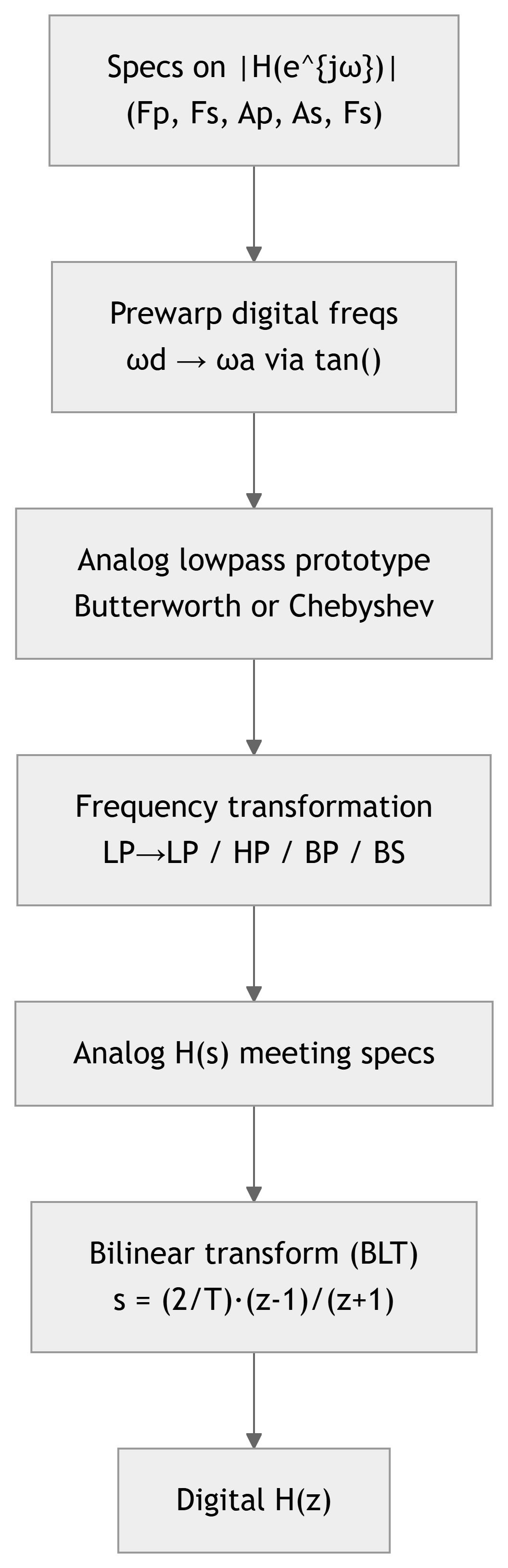
Big Picture Design Flow (BLT‑Based IIR Design)

Stress that everything in 8.3 is about steps C–D (prototype and transformation) and then BLT. Prewarping compensates BLT’s frequency nonlinearity: we map desired digital Fp, Fs back to analog ωap, ωas so that after BLT the digital edges land where we want.

8.3.1 Lowpass Prototype Functions

Idea: Design one normalized lowpass filter (prototype) with:

• Normalized passband edge: \(\nu_p = 1\)
• Specified passband ripple \(A_p\) (e.g., 3 dB, 0.5 dB, 1 dB)
• Minimal order \(n\) that also satisfies stopband attenuation \(A_s\) at \(\nu_s\)

Then:

• Transform this prototype to the desired analog filter shape (LP/HP/BP/BS).
• Convert analog \(H(s)\) → digital \(H(z)\) using BLT.

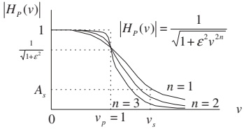
Butterworth Lowpass Prototype

Butterworth magnitude response (normalized lowpass):

\[ \left|H_P(\nu)\right| = \frac{1}{\sqrt{1 + \varepsilon^{2}\nu^{2n}}} \]

• \(\nu\): normalized frequency (prototype domain).
• \(n\): filter order.
• \(\varepsilon\): ripple parameter (for Butterworth with 3 dB spec, \(\varepsilon = 1\)).

Figure: Normalized Butterworth magnitude response

Explain that in Butterworth, the magnitude is monotonically decreasing, no ripples. For a 3‑dB LP prototype we define \(|H_P(1)|^2 = 0.5\), which implies \(\varepsilon = 1\). Discuss how higher \(n\) increases steepness of the roll‑off.

Butterworth Prototype Transfer Functions (3 dB)

From Table 8.3 (\(\varepsilon = 1\)):

\(n\)	\(H_P(s)\)
1	\(\dfrac{1}{s+1}\)
2	\(\dfrac{1}{s^{2}+1.4142s+1}\)
3	\(\dfrac{1}{s^{3}+2s^{2}+2s+1}\)
4	\(\dfrac{1}{s^{4}+2.6131s^{3}+3.4142s^{2}+2.6131s+1}\)
5	\(\dfrac{1}{s^{5}+3.2361s^{4}+5.2361s^{3}+5.2361s^{2}+3.2361s+1}\)
6	\(\dfrac{1}{s^{6}+3.8637s^{5}+7.4641s^{4}+9.1416s^{3}+7.4641s^{2}+3.8637s+1}\)

Tip

For low orders (1–6), it is common to pick \(H_P(s)\) from a table rather than factor everything by hand.

Computing Butterworth Order from Specs

Given:

• Passband ripple \(A_p\) (dB).
• Stopband attenuation \(A_s\) (dB).
• Normalized edges: \(\nu_p = 1\), \(\nu_s\) from Table 8.6.

We use:

Passband ripple:

\[ A_p\text{ dB} = -20\log_{10}\left(\frac{1}{\sqrt{1+\varepsilon^2}}\right) \]

Stopband attenuation:

\[ A_s\text{ dB} = -20\log_{10}\left(\frac{1}{\sqrt{1+\varepsilon^2\nu_s^{2n}}}\right) \]

Solving:

\[ \varepsilon^{2} = 10^{0.1A_p} - 1 \]

\[ n \ge \frac{ \log_{10}\left(\dfrac{10^{0.1A_s}-1}{\varepsilon^{2}}\right) }{ 2\log_{10}(\nu_s) } \]

Important

In practice, after computing \(n\) you always round up to the nearest integer to satisfy specs.

Chebyshev Type I Prototype (Equiripple)

Chebyshev LP prototype magnitude:

\[ \left|H_P(\nu)\right| = \frac{1}{\sqrt{1 + \varepsilon^{2} C_n^{2}(\nu)}} \]

where the (hyperbolic) Chebyshev function is:

\[ C_n(\nu) = \cosh\bigl[n \cosh^{-1}(\nu)\bigr],\quad \cosh^{-1}(x) = \ln\left(x + \sqrt{x^2 - 1}\right) \]

Figure: Normalized Chebyshev magnitude response

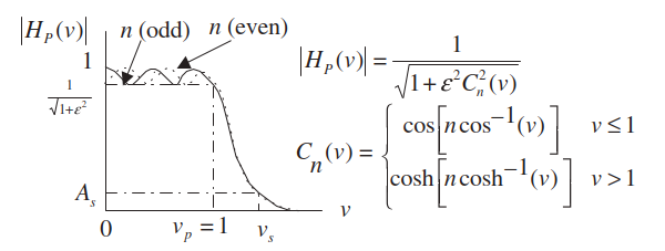
Key properties:

• Ripple in passband, monotonic stopband.
• Odd \(n\): DC gain is 1.
• Even \(n\): DC gain is \(1/\sqrt{1 + \varepsilon^2}\).
• Gain at cutoff \(\nu_p=1\) is \(1/\sqrt{1+\varepsilon^2}\) in both cases.

Explain verbally: “Chebyshev pays with passband ripples to get a narrower transition band compared to Butterworth for the same order \(n\).” Show on board a simple overlay sketch if possible.

Chebyshev Prototype Functions (Tables)

0.5 dB ripple (\(\varepsilon = 0.3493\)) – Table 8.4 (excerpt):

\(n\)	\(H_P(s)\)
1	\(\dfrac{2.8628}{s + 2.8628}\)
2	\(\dfrac{1.4314}{s^{2} + 1.4256s + 1.5162}\)
3	\(\dfrac{0.7157}{s^{3} + 1.2529s^{2} + 1.5349s + 0.7157}\)

1 dB ripple (\(\varepsilon = 0.5088\)) – Table 8.5 (excerpt):

\(n\)	\(H_P(s)\)
1	\(\dfrac{1.9652}{s + 1.9652}\)
2	\(\dfrac{0.9826}{s^{2} + 1.0977s + 1.1025}\)
3	\(\dfrac{0.4913}{s^{3} + 0.9883s^{2} + 1.2384s + 0.4913}\)

Computing Chebyshev Order from Specs

Given:

• Passband ripple \(A_p\) (dB), stopband attenuation \(A_s\) (dB).
• Normalized edges: \(\nu_p = 1\) and \(\nu_s\) from Table 8.6.

Similar to Butterworth,

\[ A_p\text{ dB} = -20\log_{10}\left(\frac{1}{\sqrt{1+\varepsilon^{2}}}\right) \quad\Rightarrow\quad \varepsilon^{2} = 10^{0.1A_p} - 1 \]

Stopband condition:

\[ A_s\text{ dB} = -20\log_{10}\left(\frac{1}{\sqrt{1+\varepsilon^{2}C_n^{2}(\nu_s)}}\right) \]

Solving for \(n\):

\[ n \ge \frac{ \cosh^{-1}\left[ \left(\dfrac{10^{0.1A_s}-1}{\varepsilon^{2}}\right)^{0.5} \right] }{ \cosh^{-1}(\nu_s) } \]

where \(\cosh^{-1}(x) = \ln(x + \sqrt{x^2 - 1})\).

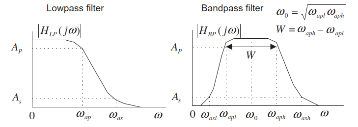
From Analog Specs to Prototype Specs

We must convert analog frequency specs \((\omega_{ap}, \omega_{as}, \dots)\) to prototype normalized frequencies.

Table 8.6 gives:

Filter	Given analog specs	Prototype specs
Lowpass	\(\omega_{ap}, \omega_{as}\)	\(\nu_p = 1,\ \nu_s = \omega_{as}/\omega_{ap}\)
Highpass	\(\omega_{ap}, \omega_{as}\)	\(\nu_p = 1,\ \nu_s = \omega_{ap}/\omega_{as}\)
Bandpass	\(\omega_{apl}, \omega_{aph}, \omega_{asl}, \omega_{ash}, \omega_0\)	\(\nu_p = 1,\ \nu_s = \dfrac{\omega_{ash}-\omega_{asl}}{\omega_{aph}-\omega_{apl}}\)
Bandstop	same parameters as bandpass	same \(\nu_s\) formula

Analog LP and BP specs

Explain each symbol on Fig. 8.15: $ {ap}$ (passband edge), $ {as}$ (stopband edge), etc. Clarify: first prewarp digital specs to analog, then convert to prototype domain via this table.

Example 8.7 – Lowpass Butterworth via BLT

Goal:

Design a digital lowpass Butterworth filter with:

1. 3‑dB attenuation at \(f_p = 1.5\) kHz.
2. 10‑dB attenuation at \(f_s = 3\) kHz.
3. Sampling frequency \(f_s = 8000\) Hz.

Example 8.7 – Step 1: Prewarping

Digital radian frequencies:

\[ \omega_{dp} = 2\pi(1500) = 3000\pi\ \text{rad/s} \]

\[ \omega_{ds} = 2\pi(3000) = 6000\pi\ \text{rad/s} \]

Sampling period:

\[ T = \frac{1}{8000}\ \text{s} \]

Apply prewarping:

\[ \omega_{ap} = \frac{2}{T}\tan\left(\frac{\omega_{dp} T}{2}\right) = 16{,}000 \tan\left(\frac{3000\pi/8000}{2}\right) \approx 1.0691\times 10^{4}\ \text{rad/s} \]

\[ \omega_{as} = \frac{2}{T}\tan\left(\frac{\omega_{ds} T}{2}\right) = 16{,}000 \tan\left(\frac{6000\pi/8000}{2}\right) \approx 3.8627\times 10^{4}\ \text{rad/s} \]

Example 8.7 – Step 2: Prototype Specs and Order

From Table 8.6 for lowpass:

\[ \nu_p = 1,\quad \nu_s = \frac{\omega_{as}}{\omega_{ap}} = \frac{3.8627\times10^{4}}{1.0691\times10^{4}} = 3.6130 \]

Given:

• Passband ripple \(A_p = 3\) dB (Butterworth 3 dB prototype).
• Stopband attenuation \(A_s = 10\) dB.

Compute:

\[ \varepsilon^{2} = 10^{0.1 \times 3} - 1 = 10^{0.3} - 1 \approx 1 \]

Order:

\[ n = \frac{\log_{10}(10^{0.1\times 10}-1)}{2\log_{10}(3.6130)} \approx 0.8553 \]

So choose \(n = 1\).

From Table 8.3:

\[ H_P(s) = \frac{1}{s+1} \]

Example 8.7 – Step 3: LP→LP and BLT

Analog LP (scale cutoff to \(\omega_{ap}\)):

\[ H(s) = H_P\left(\frac{s}{\omega_{ap}}\right) = \frac{1}{\frac{s}{\omega_{ap}} + 1} = \frac{\omega_{ap}}{s + \omega_{ap}} = \frac{1.0691\times10^4}{s + 1.0691\times10^4} \]

Apply BLT, \(s = \frac{2}{T}\frac{z-1}{z+1} = 16000\frac{z-1}{z+1}\):

\[ H(z) = \frac{1.0691\times10^4}{16000\frac{z-1}{z+1} + 1.0691\times10^4} \]

Divide numerator and denominator by 16000:

\[ H(z) = \frac{0.6682}{\frac{z-1}{z+1} + 0.6682} \]

Multiply by \((z+1)\):

\[ H(z) = \frac{0.6682(z+1)}{(z-1) + 0.6682(z+1)} = \frac{0.6682z + 0.6682}{1.6682z - 0.3318} \]

Write in \(z^{-1}\) form:

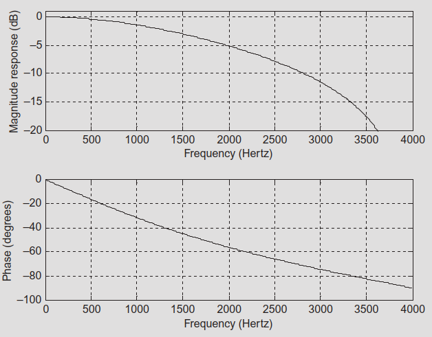
\[ H(z) = \frac{0.4006 + 0.4006z^{-1}}{1 - 0.1989z^{-1}} \]

This is a first‑order IIR digital LP filter.

Example 8.7 – MATLAB Implementation

fs = 8000;            % Sampling rate
[B, A] = lp2lp([1], [1 1], 1.0691e4);  % Step 2 (analog LP)
[b, a] = bilinear(B, A, fs);           % Step 3 (BLT)

% Numerator / denominator from MATLAB:
% b = [0.4005 0.4005];
% a = [1 -0.1989];

freqz(b, a, 512, fs);
axis([0 fs/2 -20 1]);

Frequency response Example 8.7

Point out: the 3‑dB point is near 1.5 kHz and ~10 dB attenuation near 3 kHz as specified. Encourage students to check with MATLAB or Python (scipy.signal).

Example 8.8 – Highpass Chebyshev (Order Given)

Specs:

• First‑order highpass Chebyshev type I.
• Cutoff at 3 kHz, ripple \(A_p = 1\) dB.
• Sampling frequency 8 kHz.

Example 8.8 – Key Steps

1. Prewarp the cutoff:

   \[ \omega_d = 2\pi \cdot 3000 = 6000\pi,\quad T = 1/8000 \]

   \[ \omega_a = \frac{2}{T}\tan\left(\frac{\omega_d T}{2}\right) = 16{,}000 \tan\left(\frac{6000\pi/8000}{2}\right) \approx 3.8627\times 10^4\ \text{rad/s} \]

2. Order is given: \(n=1\). Use Table 8.5 (1 dB ripple):

   \[ H_P(s) = \frac{1.9652}{s + 1.9652} \]

3. LP→HP transformation:

   \[ H(s) = H_P\left(\frac{\omega_a}{s}\right) = \frac{1.9652 s}{1.9652 s + \omega_a} \]

   Divide by 1.9652:

   \[ H(s) = \frac{s}{s + 1.9656\times 10^4} \]

4. Apply BLT → digital HP:

   \[ H(z) = \frac{s}{s + 1.9656\times 10^4} \Bigg|_{s=16000\frac{z-1}{z+1}} \]

After algebra:

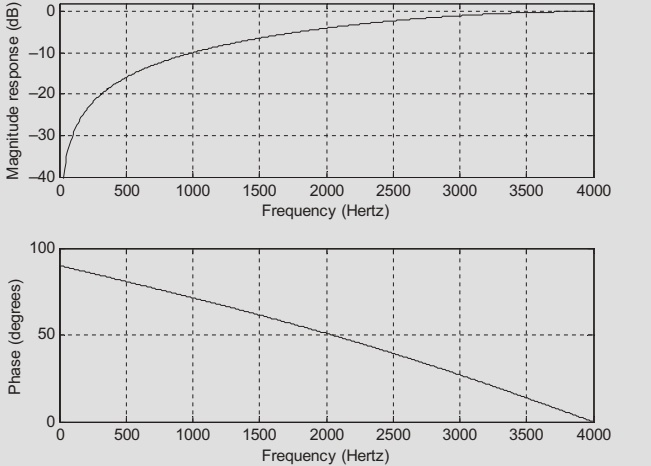
\[ H(z) = \frac{0.4487 - 0.4487 z^{-1}}{1 + 0.1025 z^{-1}} \]

Frequency response Example 8.8

Example 8.9 – Second‑Order Lowpass Butterworth

Specs:

• Second‑order LP Butterworth.
• Cutoff 3.4 kHz, \(f_s = 8000\) Hz.

Example 8.9 – Outline

1. Prewarp digital cutoff:

   \[ \omega_d = 2\pi(3400) = 6800\pi,\quad T = 1/8000 \Rightarrow \omega_a \approx 6.6645\times 10^4\ \text{rad/s} \]

2. Order given \(n=2\). Use Table 8.3:

   \[ H_P(s) = \frac{1}{s^2 + 1.4142s + 1} \]

3. LP→LP scaling:

   \[ H(s) = H_P\left(\frac{s}{\omega_a}\right) = \frac{4.4416\times 10^9}{s^2 + 9.4249\times 10^4 s + 4.4416\times 10^9} \]

4. Apply BLT:

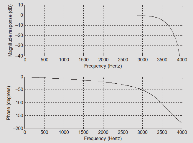
   \[ H(z) = \text{(after algebra)} = \frac{0.7157 + 1.4314z^{-1} + 0.7151z^{-2}} {1 + 1.3490z^{-1} + 0.5140z^{-2}} \]

Frequency response Example 8.9

Use this example to show a typical biquad (second‑order section). Explain that most practical IIRs are implemented as cascades of such sections for numerical stability.

Example 8.10 – Highpass Chebyshev (Order from Specs)

Specs:

• Highpass Chebyshev type I.
• Passband: 0.5 dB ripple at 3 kHz.
• Stopband: 25 dB at 1 kHz.
• \(f_s = 8000\) Hz.

We now solve for order \(n\) using Chebyshev formulas.

Example 8.10 – Steps (Condensed)

1. Prewarp:

   \[ \omega_{dp} = 6000\pi,\ \omega_{ds} = 2000\pi,\ T = 1/8000 \]

   \[ \omega_{ap} \approx 3.8627\times 10^4,\quad \omega_{as} \approx 6.6274\times 10^3 \]

2. For highpass, Table 8.6 says:

   \[ \nu_s = \frac{\omega_{ap}}{\omega_{as}} \approx 5.8284 \]

3. Compute:

   \[ \varepsilon^2 = 10^{0.1 \times 0.5} - 1 \approx 0.1220 \]

   \[ \frac{10^{0.1\cdot 25} - 1}{\varepsilon^2} \approx 2583.8341 \]

   \[ n = \frac{\cosh^{-1}\left[(2583.8341)^{0.5}\right]}{\cosh^{-1}(5.8284)} \approx 1.8875 \Rightarrow n = 2 \]

4. Choose Chebyshev prototype from Table 8.4 (\(n=2\), 0.5 dB ripple):

   \[ H_P(s) = \frac{1.4314}{s^2 + 1.4256s + 1.5162} \]

5. LP→HP transform, then BLT →

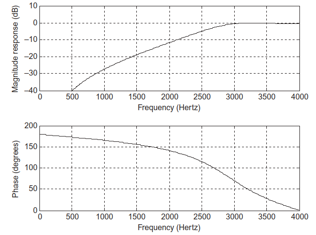
   \[ H(z) = \frac{0.1327 - 0.2654z^{-1} + 0.1327z^{-2}} {1 + 0.7996z^{-1} + 0.3618z^{-2}} \]

Frequency response Example 8.10

Bandpass / Bandstop Design Strategy

For BP and BS filters:

1. Prewarp all relevant digital edges to analog.

2. Match them to bandpass / bandstop analog specs \((\omega_{apl}, \omega_{aph}, \omega_{asl}, \omega_{ash}, \omega_0)\) and compute prototype \(\nu_s\).

3. Solve for order \(n\) (Butterworth or Chebyshev).

4. Use LP→BP or LP→BS formulas:

   • LP→BP: \(s \rightarrow \dfrac{s^2 + \omega_0^2}{Ws}\)

   • LP→BS: \(s \rightarrow \dfrac{W s}{s^2 + \omega_0^2}\)

5. Apply BLT to get digital \(H(z)\).

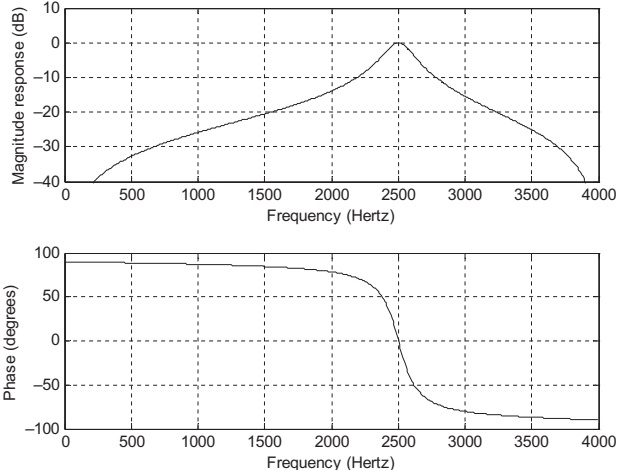
Example 8.11 – Bandpass Butterworth

Specs:

• Second‑order digital BP Butterworth.
• Lower cutoff 2.4 kHz, upper cutoff 2.6 kHz.
• \(f_s = 8000\) Hz.

Example 8.11 – Key Computations

1. Digital freqs:

   \[ \omega_h = 2\pi(2600),\quad \omega_l = 2\pi(2400),\quad T = 1/8000 \]

2. Prewarp:

   \[ \omega_{ah} \approx 2.6110\times10^4,\quad \omega_{al} \approx 2.2022\times10^4 \]

   \[ W = \omega_{ah}-\omega_{al} = 4088\ \text{rad/s} \]

   \[ \omega_0^2 = \omega_{ah}\omega_{al} \approx 5.7499\times 10^8 \]

3. Use 1st‑order prototype from Table 8.3 (\(H_P(s) = 1/(s+1)\)) so BP filter is order 2:

   LP→BP transform:

   \[ H(s) = \frac{W s}{s^2 + W s + \omega_0^2} = \frac{4088 s}{s^2 + 4088 s + 5.7499\times10^8} \]

4. BLT:

   \[ H(z) = \frac{0.0730 - 0.0730 z^{-2}}{1 + 0.7117 z^{-1} + 0.8541 z^{-2}} \]

Frequency response Example 8.11

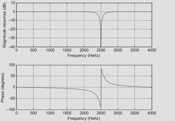
Example 8.12 – Bandstop Butterworth

Focus: - Adjusting center frequency and bandwidth so the bandstop has unity gain at \(\omega_0\) and meets passband / stopband widths. - Use LP→BS transformation and BLT.

End result (after some careful bandwidth tuning):

• Use \(n=1\) (Butterworth).

• Analog BS:

  \[ H(s) = \frac{s^{2} + 5.7341\times10^{8}}{s^{2} + 4149s + 5.7341\times10^{8}} \]

• Digital BS after BLT:

  \[ H(z) = \frac{0.9259 + 0.7078 z^{-1} + 0.9259 z^{-2}} {1 + 0.7078 z^{-1} + 0.8518 z^{-2}} \]

Frequency response Example 8.12

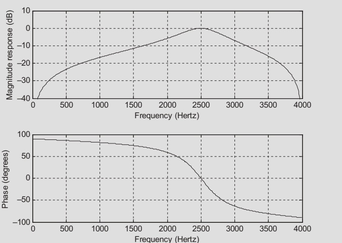
Example 8.13 – Bandpass Chebyshev

Specs:

• Center frequency 2.5 kHz.
• Passband bandwidth 200 Hz, 0.5 dB ripple.
• Stopband edges: 1.5 kHz and 3.5 kHz, 10 dB attenuation.
• \(f_s = 8000\) Hz.

Process:

• Extensive prewarping and “unit‑gain at center frequency” adjustments, then:

• Compute prototype \(\nu_s\) and order \(n\) using Chebyshev formula → \(n \approx 0.928 \Rightarrow 1\).

• Prototype from Table 8.4 (0.5 dB, \(n=1\)):

  \[ H_P(s) = \frac{2.8628}{s + 2.8628} \]

• LP→BP and BLT yield:

  \[ H(s) = \frac{1.1497\times 10^4 s}{s^{2} + 1.1497\times 10^4 s + 5.7341\times 10^8} \]

  \[ H(z) = \frac{0.1815 - 0.1815z^{-2}}{1 + 0.6264z^{-1} + 0.6396z^{-2}} \]

Frequency response Example 8.13

8.4 Higher‑Order IIR via Cascade Method

When order \(n\) is high (\(n \ge 3\)), direct‑form implementation of \(H(z)\):

• Is numerically sensitive (round‑off, coefficient quantization).
• Poles can move out of the unit circle → instability.

Solution: factor into cascaded second‑order sections (biquads).

• Each section has its own denominator \((1 + a_1 z^{-1} + a_2 z^{-2})\).
• Coefficients are better conditioned, easier to implement in hardware/embedded DSP.

Cascade Forms – Analog Prototypes

Tables 8.7–8.9 give factored lowpass prototypes.

Example: Table 8.7, 4th‑order Butterworth:

\[ H_P(s) = \frac{1}{(s^{2} + 0.7654s + 1)(s^{2} + 1.8478s + 1)} \]

Each quadratic factor → will map to one biquad in digital domain.

Chebyshev prototypes also have cascade forms (Tables 8.8, 8.9).

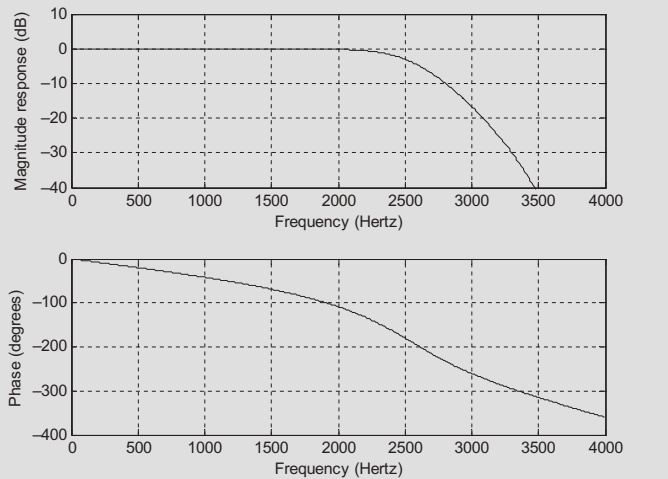
Example 8.14 – 4th‑Order Butterworth LP, Cascade

Specs:

• 4th‑order Butterworth LP.
• Cutoff 2.5 kHz.
• \(f_s = 8000\) Hz.

Example 8.14 – Steps

1. Prewarp:

   \[ \omega_d = 2\pi(2500) = 5000\pi,\quad \omega_a \approx 2.3946\times 10^4\ \text{rad/s} \]

2. Use cascade prototype from Table 8.7:

   \[ H_P(s) = \frac{1}{(s^{2} + 0.7654s + 1)(s^{2} + 1.8478s + 1)} \]

3. LP→LP for each factor:

   • First factor:

     \[ H_{P1}(s) = \frac{1}{s^{2} + 0.7654s + 1} \Rightarrow H_1(s) = H_{P1}\left(\frac{s}{\omega_a}\right) \]

   • Second factor similarly: \(H_2(s)\).

   Overall: \(H(s) = H_1(s) H_2(s)\).

4. Apply BLT to each factor:

   \[ H_1(z) = \frac{0.5108 + 1.0215z^{-1} + 0.5108z^{-2}}{1 + 0.5654z^{-1} + 0.4776z^{-2}} \]

   \[ H_2(z) = \frac{0.3730 + 0.7460z^{-1} + 0.3730z^{-2}}{1 + 0.4129z^{-1} + 0.0790z^{-2}} \]

   Overall: \(H(z) = H_1(z)H_2(z)\).

Frequency response Example 8.14

Why Cascades Are Better in Practice

Direct Form

• Single high‑order polynomial.
• Coefficient quantization can significantly alter pole locations.
• Hard to stabilize and tune.

Cascade of Biquads

• Each section 2nd‑order: \[ H_k(z) = \frac{b_{0k} + b_{1k}z^{-1} + b_{2k}z^{-2}}{1 + a_{1k}z^{-1} + a_{2k}z^{-2}} \]
• More robust to finite‑precision arithmetic.
• Easy to scale sections or change gain.

Note

Most real DSP chips (audio codecs, SDR front‑ends, etc.) include biquad building blocks specifically to implement IIR filters in cascade.

8.5 Application: Digital Audio Equalizer

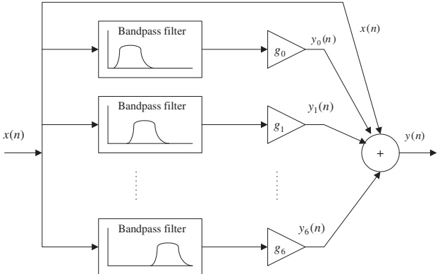
A 7‑band digital audio equalizer:

• Sampling rate \(f_s = 44.1\) kHz (CD audio).
• Audio bandwidth ~22.05 kHz.
• Each band implemented by a second‑order bandpass Butterworth filter.
• Center frequencies and bandwidths in Table 8.10.

Block diagram: audio equalizer

Audio Equalizer – Intuition

• Think of it like a graphic equalizer on a stereo.

• Each bandpass filter extracts a slice of the audio spectrum:

  • Bass (100–400 Hz).
  • Midrange (1 kHz–2.5 kHz).
  • Treble (6 kHz–15 kHz).

• Gains \(g_0, \dots, g_6\) let you boost or cut each band.

Tip

Real‑world analogy: adjusting bass and treble on your phone or car stereo is a coarse 2‑band version of this 7‑band equalizer.

Equalizer Specifications (Table 8.10)

Center freq (Hz)	100	200	400	1000	2500	6000	15000
3‑dB BW (Hz)	50	100	200	500	1250	3000	7500

Each band uses a 2nd‑order BP Butterworth IIR designed via BLT.

Table 8.11 lists the numerator/denominator coefficients \((b_k, a_k)\) for each band:

Example (Band 0):

• Numerator: \([0.0031954934, 0, -0.0031954934]\)
• Denominator: \([1, -1.9934066716, 0.9936090132]\)

Equalizer Filter Bank Responses

Magnitude responses for the seven bands

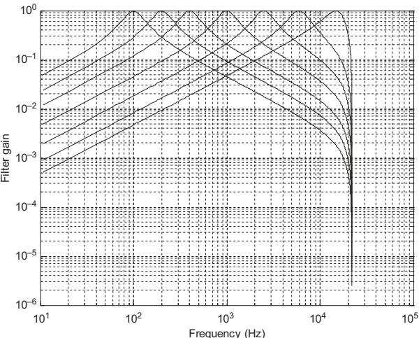
• Each curve is one bandpass filter’s gain vs frequency.
• Combined, they cover the audio band with overlapping magnitude responses.

Equalizer Operation

Input \(x(n)\) → each bandpass filter → \(y_k(n)\), then:

\[ y(n) = \left(\sum_{k=0}^{6} g_k y_k(n)\right) + x(n) \]

• The original signal is mixed back in (like a “dry + wet” mixing in audio).
• Gains \(g_k\) control emphasis per band.

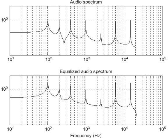
Example gain setting:

\[ g_0 = 10,\ g_1 = 10,\ g_2 = g_3 = g_4 = 0,\ g_5 = 10,\ g_6 = 10 \]

→ “Smile” EQ curve: boost very low and very high frequencies by 20 dB (\(20\log_{10}10\)), leave mids mostly unchanged.

Test Signal and Spectra

Test signal (sum of 7 sinusoids at band centers):

\[ x(n) = \sin\left(\frac{200\pi n}{44100}\right) + \sin\left(\frac{400\pi n}{44100} + \frac{\pi}{14}\right) + \cdots + \sin\left(\frac{30000\pi n}{44100} + \frac{3\pi}{7}\right) \]

Simulation shows:

• Before equalization: spectral peaks equal at each center frequency.
• After equalization: peaks at 100, 200, 6000, 15000 Hz are boosted.

Audio spectrum and equalized audio spectrum

Ask students what perceptual effect this would have: louder bass and presence, more “sparkle” in cymbals and sibilants, and relatively recessed mids (vocals/guitars).

Summary / Key Points

1. Lowpass prototypes (Butterworth & Chebyshev type I) are the starting point for many IIR designs.
2. Filter order \(n\) is determined from \(A_p, A_s\) and normalized stopband frequency \(\nu_s\).
3. Butterworth: flat passband, monotonic; Chebyshev: equiripple passband, steeper roll‑off for same order.
4. Frequency transformations map LP prototypes to LP/HP/BP/BS analog filters.
5. The bilinear transform (BLT) converts analog \(H(s)\) to digital \(H(z)\), with frequency prewarping correcting its nonlinearity.
6. Higher‑order IIR filters are best implemented as cascades of biquads for numerical robustness.
7. A multi‑band digital audio equalizer is a practical example of an IIR filter bank: each band is a 2nd‑order BP Butterworth IIR, gains adjust tonal balance.

Formula Summary

Butterworth magnitude (prototype):

\[ \left|H_P(\nu)\right| = \frac{1}{\sqrt{1 + \varepsilon^2 \nu^{2n}}} \]

Chebyshev magnitude (prototype):

\[ \left|H_P(\nu)\right| = \frac{1}{\sqrt{1 + \varepsilon^2 C_n^2(\nu)}} \]

\[ C_n(\nu) = \cosh\left[n\cosh^{-1}(\nu)\right],\quad \cosh^{-1}(x) = \ln\left(x + \sqrt{x^2 - 1}\right) \]

Ripple parameter from passband spec:

\[ \varepsilon^2 = 10^{0.1 A_p} - 1 \]

Butterworth order:

\[ n \ge \frac{\log_{10}\left(\dfrac{10^{0.1A_s} - 1}{\varepsilon^{2}}\right)} {2\log_{10}(\nu_s)} \]

Chebyshev order:

\[ n \ge \frac{\cosh^{-1}\left[\left(\dfrac{10^{0.1A_s} - 1}{\varepsilon^{2}}\right)^{0.5}\right]} {\cosh^{-1}(\nu_s)} \]

Prewarping (digital → analog):

\[ \omega_a = \frac{2}{T} \tan\left(\frac{\omega_d T}{2}\right) \]

Bilinear transform:

\[ s = \frac{2}{T}\,\frac{z - 1}{z + 1} \]

LP frequency transformations (analog domain):

• LP→LP (change cutoff): \(s \rightarrow \dfrac{s}{\omega_a}\)
• LP→HP: \(s \rightarrow \dfrac{\omega_a}{s}\)
• LP→BP: \(s \rightarrow \dfrac{s^2 + \omega_0^2}{W s}\)
• LP→BS: \(s \rightarrow \dfrac{W s}{s^2 + \omega_0^2}\)

IIR Filter Design – Interactive Deck

How to Use This Interactive Deck

• You can edit and run Python code directly in many slides.
• Code blocks tagged {pyodide} run in your browser using Pyodide (Python in WebAssembly).
• Some slides use Observable JS (OJS) + Pyodide + Plotly for reactive visualizations.
• Try changing parameters (e.g., \(A_p, A_s, n\)) and see how filter behavior changes immediately.

Tip

Click inside a code cell, modify values, then press the Run button (or use the keyboard shortcut if available) to re‑execute.

Warm‑up: dB and Linear Gain

Play with the basic conversion between dB and linear gain.

Encourage students to try Ap = 0.5 and Ap = 3, then ask them what happens to the linear passband ripple.

Computing the Butterworth Ripple Parameter ϵ

From the lecture:

\[ \varepsilon^{2} = 10^{0.1A_p} - 1 \]

Use this block to experiment with different passband ripples \(A_p\).

Try adding another \(A_p\) value (e.g., 0.1 dB) to the list and rerun.

Butterworth Order Calculator (Interactive)

Recall Butterworth order formula:

\[ n \ge \frac{\log_{10}\left(\dfrac{10^{0.1A_s} - 1}{\varepsilon^{2}}\right)} {2\log_{10}(\nu_s)},\quad \varepsilon^{2} = 10^{0.1A_p} - 1 \]

Use this interactive calculator to see how \(A_p, A_s, \nu_s\) affect the required order.

Task: Change Ap, As, and nu_s and see how the minimum integer order changes.

Reactive Butterworth Order Explorer

Use sliders (OJS) to control \(A_p\), \(A_s\), and \(\nu_s\), and get the order and a quick visualization of the transition region.

viewof Ap = Inputs.range([0.1, 3], {step: 0.1, value: 1, label: "Passband ripple Ap (dB)"})
viewof As = Inputs.range([10, 60], {step: 5, value: 30, label: "Stopband attenuation As (dB)"})
viewof nu_s = Inputs.range([1.1, 5], {step: 0.1, value: 2, label: "Normalized stopband edge ν_s"})

Ask: “What happens to \(n\) when you demand very small ripple (Ap → 0.1 dB) and very high attenuation (As → 60 dB) with a small separation (νs near 1.2)?”

Chebyshev Order Calculator (Interactive)

Chebyshev order:

\[ n \ge \frac{\cosh^{-1}\left[\left(\dfrac{10^{0.1A_s}-1}{\varepsilon^{2}}\right)^{0.5}\right]} {\cosh^{-1}(\nu_s)},\quad \varepsilon^{2} = 10^{0.1A_p} - 1 \]

Try adjusting Ap, As, and nu_s and compare with Butterworth for same specs.

Butterworth vs Chebyshev Order – Reactive Comparison

Use sliders to compare required orders for the same specs.

viewof Ap_common = Inputs.range([0.1, 3], {step: 0.1, value: 1, label: "Ap (dB), both filters"})
viewof As_common = Inputs.range([10, 80], {step: 5, value: 40, label: "As (dB), both filters"})
viewof nu_s_common = Inputs.range([1.1, 5], {step: 0.1, value: 2, label: "ν_s, both filters"})

Highlight that Chebyshev typically achieves the same specs with lower order (especially for tough specs), at the cost of passband ripple.

Prewarping Digital Frequency to Analog

Prewarping formula:

\[ \omega_a = \frac{2}{T} \tan\left(\frac{\omega_d T}{2}\right), \quad T = \frac{1}{f_s},\ \omega_d = 2\pi f_d \]

Experiment with the prewarped analog cutoff for different sampling rates and digital cutoff frequencies.

Try adding other fs values (e.g., 16000, 48000) and see how \(\omega_a\) changes.

Visualizing Prewarping Nonlinearity

Plot mapping from digital frequency \(f_d\) to prewarped analog \(\omega_a\) for a given \(f_s\).

Observe how mapping becomes steeper near Nyquist (\(f_s/2\)).

Interactive: Example 8.7 Design in Python

Approximate Example 8.7 using Python tools for filter design (scipy‑like pattern, but we will only compute formulas here).

Change Ap or As and see whether an order of 1 is still enough.

Simple Butterworth Analog Prototype Plot (Magnitude Only)

Plot the normalized Butterworth magnitude response for a given order \(n\).

Experiment by changing n and Ap and rerun to see the effect on roll‑off and passband.

Chebyshev Prototype Magnitude Plot (Approximate)

Approximate Chebyshev type I magnitude using numpy.polynomial.chebyshev.chebval for \(|ν| \le 1\) and hyperbolic extension for \(|ν|>1\).

Try different n and Ap and compare with the Butterworth prototype slide.

Reactive: Try Your Own Lowpass Specs

Use sliders to specify a lowpass analog filter (already prewarped) and see normalized prototype stopband and required Butterworth order.

viewof omega_ap = Inputs.range([1000, 50000], {step: 1000, value: 5000, label: "Analog passband edge ω_ap (rad/s)"})
viewof omega_as = Inputs.range([2000, 100000], {step: 2000, value: 20000, label: "Analog stopband edge ω_as (rad/s)"})
viewof Ap_lp = Inputs.range([0.1, 3], {step: 0.1, value: 1, label: "Ap (dB)"})
viewof As_lp = Inputs.range([10, 60], {step: 5, value: 40, label: "As (dB)"})

Interactive Audio Equalizer – Conceptual Numeric Play

We will not process full audio here, but we can explore gains per band and resulting total gain at each center frequency.

Center frequencies (Table 8.10):

• [100, 200, 400, 1000, 2500, 6000, 15000] Hz

viewof g0 = Inputs.range([0, 10], {step: 1, value: 10, label: "g0 (100 Hz)"})
viewof g1 = Inputs.range([0, 10], {step: 1, value: 10, label: "g1 (200 Hz)"})
viewof g2 = Inputs.range([0, 10], {step: 1, value: 0,  label: "g2 (400 Hz)"})
viewof g3 = Inputs.range([0, 10], {step: 1, value: 0,  label: "g3 (1 kHz)"})
viewof g4 = Inputs.range([0, 10], {step: 1, value: 0,  label: "g4 (2.5 kHz)"})
viewof g5 = Inputs.range([0, 10], {step: 1, value: 10, label: "g5 (6 kHz)"})
viewof g6 = Inputs.range([0, 10], {step: 1, value: 10, label: "g6 (15 kHz)"})

Try making your own EQ curve (e.g., mid‑boost, treble‑cut) and relate it to how music would sound.

Mini‑Challenge 1

Use any of the calculators above to design:

• A Butterworth LP with:
  • \(A_p = 1\) dB, \(A_s = 40\) dB,
  • \(\nu_s = 2.5\).

Then:

1. Compute the order \(n\) with the Butterworth calculator.
2. Design a Chebyshev type I with the same specs and compute its order.
3. Which one has the lower order?

Use both:

• The simple order calculator slides.
• The comparison slide (Butterworth vs Chebyshev).

Mini‑Challenge 2 – Move from Specs to Prototype

Pick analog LP specs:

• \(\omega_{ap} = 10{,}000\ \text{rad/s}\),
• \(\omega_{as} = 30{,}000\ \text{rad/s}\),
• \(A_p = 1\) dB, \(A_s = 25\) dB.

Tasks:

1. Use the “Try Your Own Lowpass Specs” slide to find \(\nu_s\) and Butterworth order \(n\).
2. Change \(A_p\) from 1 dB → 0.1 dB and observe how \(n\) changes.
3. Reflect: why does tightening passband ripple increase the required order?

Write your answers (and screenshots if possible) in your lab notebook.

Wrap‑Up: Key Takeaways from the Interactive Deck

• You can now compute filter order for both Butterworth and Chebyshev I IIR filters from \((A_p, A_s, \nu_s)\).

• You’ve seen how prewarping adjusts analog specs before BLT.

• You used live Python code to:

  • Implement the formulas for \(\varepsilon\), \(n\), and prewarped \(\omega_a\).
  • Visualize magnitude responses of Butterworth and Chebyshev prototypes.

• You explored how a multi‑band equalizer is essentially a bank of bandpass IIR filters plus gains.

Tip

Keep this deck open while doing homework: copy the formulas, tweak the code, and use it as a design sandbox.