7.2 FIR Filter Design – Applications & Advanced Methods
Digital Signal Processing
Learning Objectives
By the end of this session, you should be able to:
Explain how FIR filters are used for noise reduction in:
Single‑tone measurement signals
Speech signals
Vibration signals in mechanical systems
Describe and sketch the signal flow for a two‑band digital audio crossover.
Use the frequency sampling method to design a linear‑phase FIR filter given sampled magnitude specs.
Interpret how smooth transition bands affect ripple (Gibbs phenomenon).
Describe the Parks–McClellan (optimal) method conceptually and follow its step‑by‑step design procedure.
Choose an appropriate FIR design method (window, frequency sampling, optimal) for a given application.
This lecture assumes students have already seen: - Basic FIR structure and impulse response - Window method for FIR design - Basic DFT/IDFT relationships
We now connect FIR design to real applications (noise reduction, audio) and introduce two more powerful design methods: frequency sampling and optimal (Parks–McClellan).
7.4 Applications: Noise Reduction & Two‑Band Digital Crossover
We now look at FIR filters in real ECE contexts:
Measurement and instrumentation (cleaning a single sine in broadband noise)
Speech systems (telephone / VoIP)
Vibration monitoring (rotating machines, structures)
Audio systems (woofer + tweeter crossover)
Think of FIR filters as “frequency‑selective sieves” :
We keep the frequency band where the useful information lies.
We attenuate the rest as “noise” or unwanted content.
7.4.1 Noise Reduction – Measurement Signal
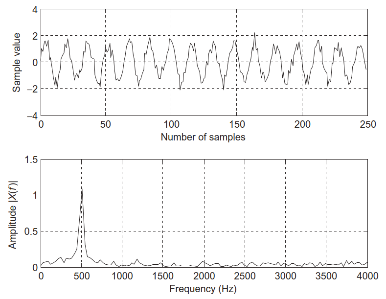
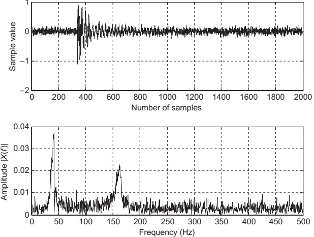
We measure a 500 Hz sine at sampling rate \(f_s = 8000\) Hz:
\[
x(n)=1.4141\sin\left(\frac{2\pi\cdot500n}{8000}\right)+\nu(n)
\]
\(\nu(n)\) : broadband Gaussian noise, 0–4000 Hz.Assume the desired signal energy lies only between 0–800 Hz.
So frequencies above 800 Hz are treated as noise.
Filter specs (lowpass FIR):
Passband: 0–800 Hz, ripple \(< 0.02\) dB
Stopband: 1000–4000 Hz, attenuation \(\ge 50\) dB
Top: noisy 500 Hz sine in time domain
Bottom: magnitude spectrum – clear tone at 500 Hz plus broadband noise up to 4 kHz
Emphasize:
500 Hz sine is within our desired band.
Random noise spreads across all frequencies.
We use prior knowledge: “my signal of interest is low‑frequency.”
Passband/stopband numbers are engineering specs: passband ripple and stopband attenuation are performance metrics for the filter.
Noise Reduction – FIR Design & Result
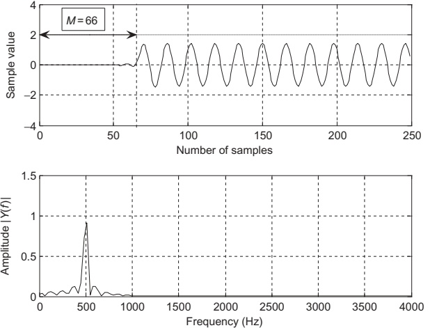
Using the window method with a Hamming window :
Cutoff frequency \(f_c=900\) Hz (slightly above 800 Hz passband).
Filter length \(N=133\) taps (from design tables, e.g., Table 7.7 in text).
Key outcomes:
Noise strongly reduced in 1000–4000 Hz region.Remaining noise within passband (0–800 Hz) cannot be removed by this filter.
Because \(N=133\) , linear‑phase group delay is \[
\text{delay} = \frac{N-1}{2} = 66\text{ samples}
\]
Transient response lasts first \(N-1=132\) samples.
Time plot: delayed but much cleaner 500 Hz sinusoid.
Spectrum: near‑zero noise from 1–4 kHz; some “shoulders” 400–700 Hz (in‑band noise that remains).
Engineering Insight – What Filtering Can & Can’t Do
A lowpass FIR can remove out‑of‑band noise (e.g., > 1 kHz).
It cannot remove noise that overlaps the desired signal in frequency (e.g., 400–700 Hz here).
Point out that real filters have finite transition bands; we set \(f_c=900\) Hz to get desired in‑band/stopband trade‑off.
Also emphasize delay and transient: this is why real‑time systems sometimes compensate for delay or use shorter filters.
7.4.2 Speech Noise Reduction
Scenario:
Speech recorded at \(f_s=8000\) Hz in a noisy environment.
Typical speech energy is concentrated below ~3–4 kHz.
Here we assume useful information is within 0–1800 Hz .
FIR lowpass specs:
Type: lowpass FIR, linear phase
Passband: 0–1800 Hz, ripple \(< 0.02\) dB
Stopband: 2000–4000 Hz, attenuation \(\ge 50\) dB
Design parameters (from tables):
Window: Hamming
\(N=133\) tapsCutoff \(f_c = 1900\) Hz
Goal: remove high‑frequency broadband noise (e.g., hiss) while keeping consonants and vowel formants mostly intact.
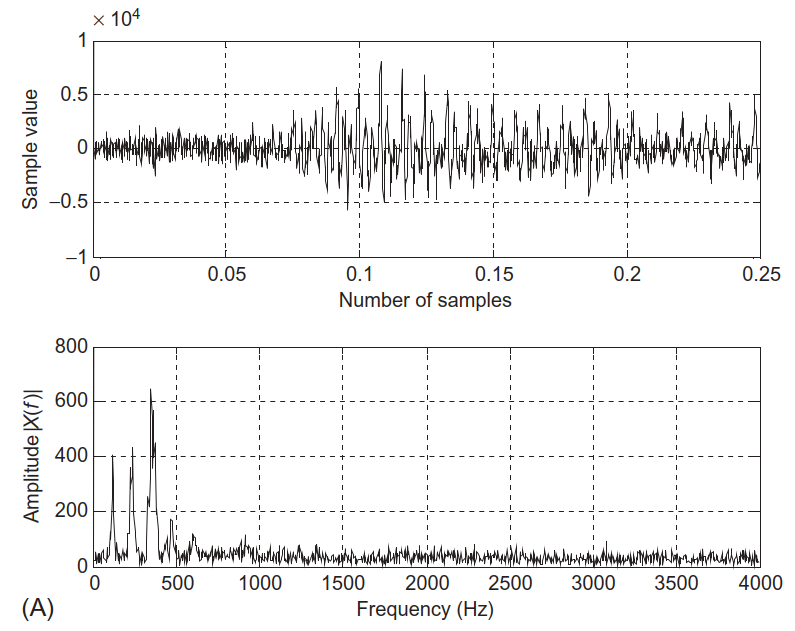
Time: noisy speech waveform.
Spectrum: high‑level broadband noise, especially above 2 kHz.
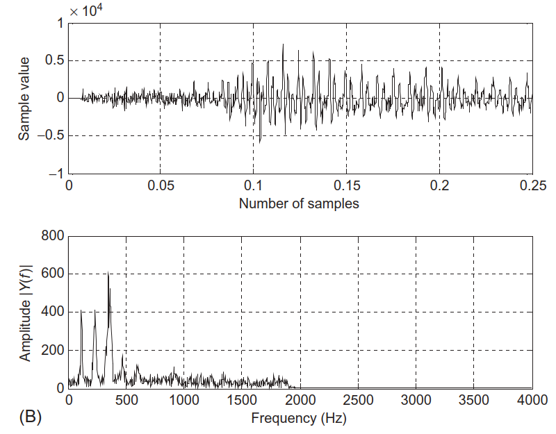
Time: enhanced (cleaner) speech.
Spectrum: noise above 2 kHz greatly reduced.
Relate to telephone bandwidth (300–3400 Hz). Here we are stricter (up to 1.8 kHz) to obtain good noise reduction.
Highlight application: VoIP pre‑processing, speech recognition front‑ends, hearing aids – all use similar filtering ideas.
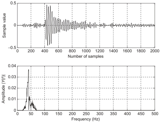
7.4.3 Noise Reduction in Vibration Signals
Vibration analysis setup:
Accelerometer signal sampled at \(f_s = 1000\) Hz.
Dominant vibration component expected in 35–50 Hz (e.g., gear mesh, rotor frequency).
Signal heavily corrupted by broadband noise.
Bandpass FIR specs:
Passband: 35–50 Hz, ripple \(< 0.02\) dB
Stopbands: 0–15 Hz and 70–500 Hz, attenuation \(\ge 50\) dB
Design chosen:
Window: Hamming
\(N=167\) tapsLow cutoff: 25 Hz
High cutoff: 60 Hz
Goal: isolate the first dominant vibration mode while suppressing low‑frequency drift and high‑frequency noise.
In mechanical / structural health monitoring, clean band‑limited vibration is crucial for:
Condition‑based maintenance (detect bearing faults).
Modal analysis (identify resonant frequencies).
Fault detection in rotating machinery (motors, turbines).
Emphasize that bandpass filters can be seen as “zooming” into a narrow frequency band of interest, analogous to tuning a radio station.
Students should recognize that exactly the same FIR theory applies across audio, speech, vibration, etc. Only the frequency scales change.
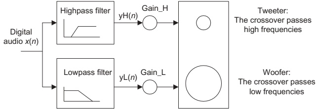
7.4.4 Two‑Band Digital Crossover – Audio Application
In loudspeaker systems:
No single driver (cone, tweeter) can handle the entire 20 Hz–20 kHz range well.
Use multiple drivers:
Woofer – low frequenciesTweeter – high frequencies
A two‑band digital crossover splits the input into:
Low band → amplified → woofer
High band → amplified → tweeter
Requirements:
Combined magnitude response must be flat across the audio band.
Sharp transitions around the crossover frequency to avoid distortion and overlap.
Prefer linear phase (FIR) for minimal phase distortion in audio.
One digital input.
Parallel lowpass + highpass FIR filters.
Separate amplifiers and speaker drivers.
Connect to real life: studio monitors, Bluetooth speakers, car audio – almost all multiway loudspeakers use analog or digital crossovers internally.
Digital crossovers are attractive because we can easily change crossover frequency, slopes, and phase alignment in software.
Digital Crossover Specifications
Given:
Sampling rate: \(f_s = 44100\) Hz (CD audio).
Crossover (cutoff) frequency: \(f_c = 1000\) Hz.
Transition band: 600–1400 Hz.
Lowpass FIR:
Passband: 0–600 Hz, ripple \(< 0.02\) dB
Stopband edge: 1400 Hz, attenuation \(\ge 50\) dB
Highpass FIR:
Passband: 1400–22050 Hz (up to Nyquist), ripple \(< 0.02\) dB
Stopband edge: 600 Hz, attenuation \(\ge 50\) dB
Design decision:
Use Hamming window FIR for both lowpass and highpass.
Transition width: \(800\) Hz → from design tables → \(N=183\) taps.
Both filters share the same cutoff frequency \(f_c = 1000\) Hz, ensuring complementary magnitude responses.
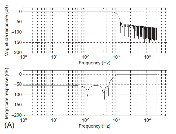
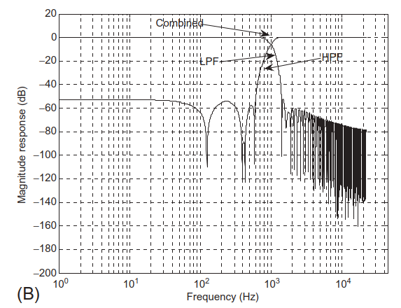
Crossover Frequency Responses
Magnitude responses of lowpass and highpass filters individually.
Both cross at 1000 Hz.
Lowpass + highpass + combined magnitude response.
Combined response is essentially flat across all frequencies.
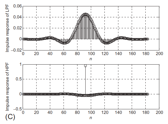
Impulse responses (FIR coefficients) of both filters.
To get a flat crossover , the lowpass and highpass magnitude responses must be complementary around \(f_c\) :
At each frequency in the transition band, \(|H_\text{LP}(f)|^2 + |H_\text{HP}(f)|^2 \approx 1\) (if normalized).
Discuss group delay: both filters are length 183, so they have identical delay \((N-1)/2\) , preserving time alignment between woofer and tweeter.
Mention that IIR crossovers (e.g., Linkwitz–Riley) are common too; FIR gives more precise control and linear phase at the cost of longer delay.
7.5 Frequency Sampling Design Method – Idea
We now move from window method to frequency sampling .
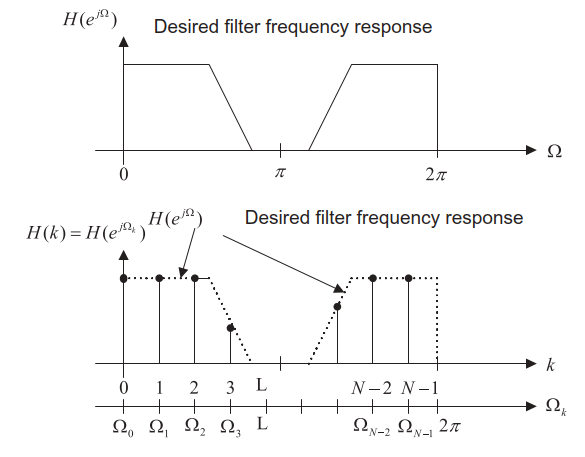
Key idea:
Directly specify the desired magnitude response at a set of equally spaced frequencies , then use IDFT to obtain \(h(n)\) .
Think of it as:
“Draw the magnitude response you want, sample it at DFT frequencies, then invert the DFT to get the impulse response.”
Let:
\(h(n)\) , \(n=0,\dots,N-1\) = FIR coefficients (causal).\(H(k)\) , \(k=0,\dots,N-1\) = DFT of \(h(n)\) .
Relationship:
\[
H(k) = H\!\left(e^{j\Omega_k}\right), \quad \Omega_k = \frac{2\pi k}{N}
\]
We prescribe \(H(k)\) by prescribing \(H(e^{j\Omega_k})\) at these grid points.
DFT/IDFT Connection
Given FIR transfer function:
\[
H(z)=h(0)+h(1)z^{-1}+\cdots+h(N-1)z^{-(N-1)}
\]
Frequency response:
\[
H\!\left(e^{j\Omega}\right)=\sum_{n=0}^{N-1}h(n)e^{-jn\Omega}
\]
Sample at \(\Omega_k = 2\pi k/N\) :
\[
H\!\left(e^{j\Omega_k}\right)
=
\sum_{n=0}^{N-1}h(n)e^{-j\frac{2\pi}{N}kn}
=
\sum_{n=0}^{N-1}h(n)W_N^{nk}
= H(k)
\]
where \(W_N = e^{-j2\pi/N}\) .
So:
\(H(k)\) is just the DFT of \(h(n)\) .Therefore \(h(n)\) is the IDFT of \(H(k)\) :
\[
h(n) = \frac{1}{N}\sum_{k=0}^{N-1} H(k) W_N^{-kn}
\]
Frequency sampling method = Design in frequency domain, compute in time domain via IDFT .
Stress that we are free to choose \(H(k)\) as long as we ensure Hermitian symmetry (for real \(h(n)\) ) and optionally linear phase (via symmetric \(h(n)\) ).
Linear phase is optional; the basic derivation doesn’t assume it.
Ensuring Real Coefficients – Symmetry in \(H(k)\)
We want \(h(n)\) real.
For real \(h(n)\) , the DFT satisfies conjugate symmetry :
\[
H(N-k)=\overline{H(k)}
\]
Using this property, we can write:
\[
h(n)
=
\frac{1}{N}
\left[
H(0) + 2\Re\left\{
\sum_{k=1}^{M} H(k) W_N^{-kn}
\right\}
\right],
\quad N=2M+1
\]
This equation reduces computation and ensures \(h(n)\in\mathbb{R}\) .
Adding Linear Phase – Symmetric \(h(n)\)
For Type I linear‑phase FIR (odd length \(N=2M+1\) , symmetric \(h(n)\) ):
\[
h(n) = h(2M-n),\quad 0\le n\le 2M
\]
We can express \(H(e^{j\Omega})\) as:
\[
H\!\left(e^{j\Omega}\right)
=
e^{-jM\Omega}
\left[
h(M) +
\sum_{n=1}^{M-1} 2h(n)\cos\big[(M-n)\Omega\big]
\right]
\]
The bracketed term is real (magnitude), and \(e^{-jM\Omega}\) gives linear phase.
We sample at \(\Omega_k = \frac{2\pi k}{N}\) and specify real magnitudes \(H_k\) :
\[
H\!\left(e^{j\Omega_k}\right) =
H_k e^{-j\frac{2\pi}{N}kM} = H(k)
\]
Substituting into IDFT and simplifying, we get the design formula for \(0\le n\le M\) :
\[
h(n) = \frac{1}{N}\left[
H_0 + 2\sum_{k=1}^{M} H_k
\cos\left(
\frac{2\pi k(n-M)}{2M+1}
\right)
\right]
\]
Then extend using symmetry:
\[
h(n) = h(2M-n),\quad n=M+1,\dots,2M
\]
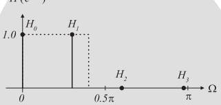
Example 7.12 – 7‑Tap Lowpass via Frequency Sampling
Design:
\(N=7\Rightarrow 2M+1=7\Rightarrow M=3\) .Cutoff frequency \(\Omega_c = 0.3\pi\) rad.
Sampled frequencies:
\[
\Omega_k = \frac{2\pi}{7}k,\quad k=0,1,2,3
\]
Specify magnitudes (lowpass‑like):
\(H_0 = 1\) at \(\Omega_0=0\) \(H_1 = 1\) at \(\Omega_1 = \frac{2\pi}{7}\) \(H_2 = 0\) at \(\Omega_2 = \frac{4\pi}{7}\) \(H_3 = 0\) at \(\Omega_3 = \frac{6\pi}{7}\)
Using design formula:
\[
\begin{aligned}
h(n)
&=
\frac{1}{7}\left[
1 + 2\sum_{k=1}^{3}H_k\cos\left(\frac{2\pi k(n-3)}{7}\right)
\right],\ n=0,1,2,3\\
&=
\frac{1}{7}\left[
1 + 2\cos\left(\frac{2\pi(n-3)}{7}\right)
\right]
\end{aligned}
\]
since \(H_2=H_3=0\) .
Computed coefficients:
\(h(0) = -0.11456\) \(h(1) = 0.07928\) \(h(2) = 0.32100\) \(h(3) = 0.42857\)
By symmetry:
\(h(4)=h(2)\) , \(h(5)=h(1)\) , \(h(6)=h(0)\) .
This is a very compact way to generate linear‑phase FIR coefficients from a small vector of frequency samples \(H_k\) .
MATLAB Helper – firfs(N,Hk)
The text supplies a MATLAB function:
function B = firfs (N , Hk )% B=firfs(N,Hk) % FIR filter design using the frequency sampling method. % Input: % N : number of filter coefficients (must be odd). % Hk : vector of sampled frequency response for k=0,...,M=(N-1)/2. % Output: % B : FIR filter coefficients (length N). Usage:
Provide odd \(N\) and vector \(Hk=[H_0,H_1,\dots,H_M]\) .
firfs computes \(h(n)\) for \(n=0,\dots,N-1\) using the formula we derived.
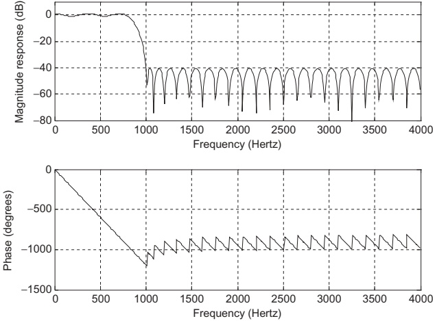
Reducing Ripple – Smooth Transition Band
To reduce Gibbs oscillations, modify \(H_k\) to have a smooth transition :
\[
H_k = [1\,1\,1\,1\,1\,1\,0.5\,0\,0\,0\,0\,0]
\]
Use firfs again:
H2 = [1 1 1 1 1 1 0.5 0 0 0 0 0 ]; B2 = firfs (25 , H2 ); h2 , f ] = freqz (B2 , 1 , 512 , fs );
Dash‑dotted: abrupt transition → strong ripples.
Solid: smoother transition in \(H_k\) → reduced ripples.
Table 7.12 lists coefficients for both designs.
Trade‑off:
Sharper transitions in the desired magnitude specification → more ripples (Gibbs).
Smoother transitions → less ripple but wider actual transition band.
MATLAB design (Program 7.9 skeleton):
fs = 8000 ; H1 = [0 0 0 1 1 1 1 0 0 0 ]; % ideal-ish B1 = firfs (25 , H1 ); h1 , w ] = freqz (B1 , 1 , 512 ); H2 = [0 0 0 0.5 1 1 1 1 0.5 0 0 0 ]; % smoothed B2 = firfs (25 , H2 ); h2 , w ] = freqz (B2 , 1 , 512 );
Again:
Dash‑dotted: abrupt transitions → stronger ripple.
Solid: smoothed transitions → reduced ripple.
Coefficients are in Table 7.13.
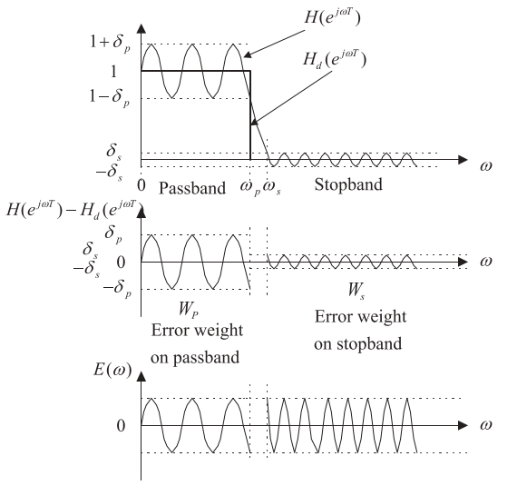
7.6 Optimal Design: Parks–McClellan Algorithm
We now consider a more advanced, widely used method:
Goal: Minimize the maximum error between desired and actual magnitude response → minimax (Chebyshev) optimization.Result: Equiripple FIR filters – ripples are equal in magnitude across the passband and stopband.
Let:
\(H_d(e^{j\omega T})\) : ideal desired magnitude response.\(H(e^{j\omega T})\) : actual FIR response.\(W(\omega)\) : weighting function to emphasize/de‑emphasize certain bands.
Error function:
\[
E(\omega) = W(\omega)\left[
H(e^{j\omega T}) - H_d(e^{j\omega T})
\right]
\]
We seek to minimize:
\[
\min \left( \max_\omega |E(\omega)| \right)
\]
The algorithm uses Remez exchange and Chebyshev polynomials internally (details beyond this course).
Top:
Ideal lowpass vs practical equiripple FIR (Parks–McClellan).
Passband ripple \(\delta_p\) , stopband ripple \(\delta_s\) .
Middle:
Error (unweighted) in passband and stopband.
If one band has much larger error, optimization is unbalanced.
Bottom:
Weighted error with \(W_p\) (passband) and \(W_s\) (stopband).
We choose \(W_p\) and \(W_s\) so that weighted errors are about equal across bands.
Conversions from dB specs:
\[
\delta_p = 10^{\frac{\delta_p\text{(dB)}}{20}} - 1
\]
\[
\delta_s = 10^{\frac{\delta_s\text{(dB)}}{20}}
\]
Then:
\[
\frac{\delta_p}{\delta_s} = \frac{W_s}{W_p} = \frac{\text{numerator}}{\text{denominator}}
\]
So:
Choose integer ratio \(\approx \delta_p/\delta_s\) , set \(W_s = \text{numerator}\) , \(W_p = \text{denominator}\) .
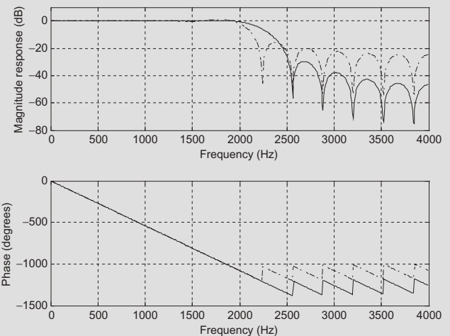
Example 7.15 – Lowpass via Parks–McClellan
Specs:
\(f_s = 8000\) Hz.Passband: 0–800 Hz, ripple \(\le 1\) dB.
Stopband: 1000–4000 Hz, attenuation \(\ge 40\) dB.
Filter order: 53 (→ 54 taps).
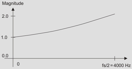
Normalize by \(f_s/2=4000\) Hz:
0 Hz → 0, magnitude 1
800 Hz → \(0.2\) , magnitude 1
1000 Hz → \(0.25\) , magnitude 0
4000 Hz → 1, magnitude 0
Weights:
\[
\delta_p = 10^{\frac{1}{20}} - 1 \approx 0.1220
\]
\[
\delta_s = 10^{\frac{-40}{20}} = 0.01
\]
Ratio:
\[
\frac{\delta_p}{\delta_s} \approx 12.2 \approx \frac{12}{1} = \frac{W_s}{W_p}
\]
So \(W_s = 12\) , \(W_p = 1\) .
MATLAB (Program 7.10):
fs = 8000 ; f = [0 0.2 0.25 1 ]; % band edges (normalized) m = [1 1 0 0 ]; % ideal mags w = [1 12 ]; % weights [passband stopband] b = firpm (53 , f , m , w ); % 54-tap equiripple FIR freqz (b , 512 , fs ); axis ([0 fs / 2 - 80 10 ]);
Results:
Stopband attenuation meets 40 dB requirement.
Zoomed‑in passband (Fig. 7.35) shows ripples between −1 dB and +1 dB → meets spec.
Coefficients are symmetric (Table 7.14).
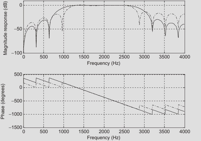
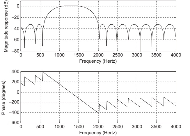
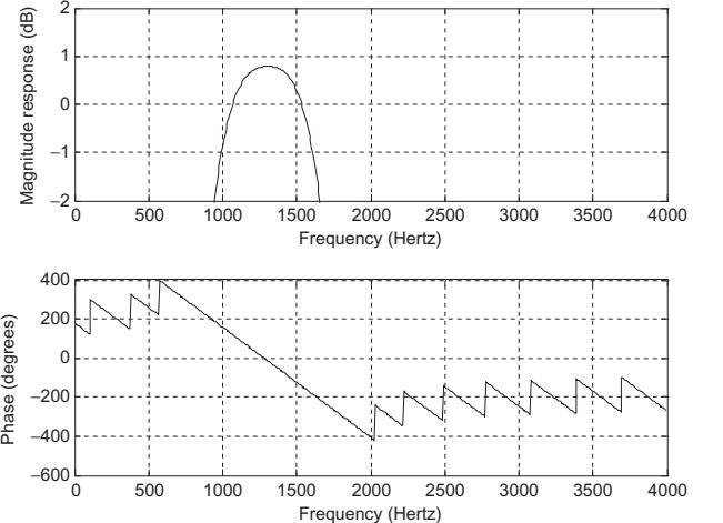
Example 7.16 – Bandpass via Parks–McClellan
Specs:
\(f_s=8000\) Hz.Passband: 1000–1600 Hz (1 dB ripple).
Stopbands: 0–600 Hz and 2000–4000 Hz (30 dB attenuation).
Filter order: 25 (26 taps).
Normalize by 4000 Hz:
0 Hz → 0, magnitude 0
600 Hz → 0.15, magnitude 0
1000 Hz → 0.25, magnitude 1
1600 Hz → 0.4, magnitude 1
2000 Hz → 0.5, magnitude 0
4000 Hz → 1, magnitude 0
Weights:
\[
\delta_p = 10^{\frac{1}{20}} - 1 \approx 0.1220,\quad
\delta_s = 10^{\frac{-30}{20}} \approx 0.0316
\]
Ratio:
\[
\frac{\delta_p}{\delta_s} \approx 3.86 \approx \frac{39}{10}
=
\frac{W_s}{W_p}
\]
So \(W_s=39\) , \(W_p=10\) .
MATLAB (Program 7.11):
fs = 8000 ; f = [0 0.15 0.25 0.4 0.5 1 ]; m = [0 0 1 1 0 0 ]; w = [39 10 39 ]; % [lower stop, pass, upper stop] b = firpm (25 , f , m , w ); freqz (b , 512 , fs ); axis ([0 fs / 2 - 80 10 ]);
Results:
Stopband attenuation meets ≥30 dB.
Passband ripple between −1 dB and +1 dB (Fig. 7.37).
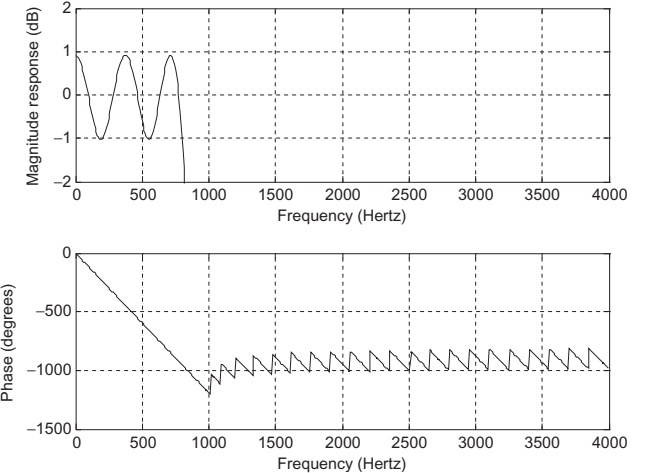
Example 7.17 – Remez Exchange on a 3‑Tap Filter
This example shows how the Remez algorithm iteratively adjusts coefficients to achieve equiripple error.
Filter structure (Type I linear phase):
\[
H(z) = b_0 + b_1 z^{-1} + b_0 z^{-2}
\]
Frequency response magnitude (ignoring linear phase):
\[
H(e^{j\Omega}) = b_1 + 2b_0\cos\Omega
\]
Desired magnitude \(H_d(e^{j\Omega})\) :
Increases linearly from 0.5 at \(\Omega=0\) to 1 at \(\Omega=\pi/4\) .
Transition band from \(\pi/4\) to \(\pi/2\) .
Decreases linearly from 0.75 at \(\Omega=\pi/2\) to 0 at \(\Omega=\pi\) .
Set weight \(W(\Omega)=1\) .
Error:
\[
E(\Omega) = H(e^{j\Omega}) - H_d(e^{j\Omega})
\]
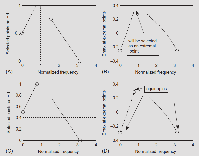
Remez alternation theorem:
There must be at least \(M+2\) extremal frequencies for an \(M\) ‑th degree Chebyshev approximation.
Here degree is 1 in \(\cos\Omega\) → need 3 extremal frequencies.
At extremal frequencies \(\Omega_k\) , error alternates sign and has equal magnitude \(E_{\max}\) .
After two iterations, they obtain:
\[
H(z) = 0.125 + 0.537 z^{-1} + 0.125 z^{-2}
\]
with equiripple error amplitude ≈ 0.287.
You don’t need to reproduce this derivation by hand in exams; the goal is to understand conceptually how Remez finds optimal equiripple filters.
Tools like MATLAB’s firpm implement all of this internally.
Summary: Comparing FIR Design Methods
From Section 7.10 and Table 7.19:
Window (Fourier + window)
LP, HP, BP, BS (standard shapes)
Yes
Used to choose order; must check
Moderate (closed‑form + window)
Calculator or simple code
Frequency Sampling
Any magnitude shape
Yes (if symmetric) or no (if not)
Specs checked a posteriori
Simple (single formula)
Calculator or MATLAB
Optimal (Parks–McClellan)
Any type
Yes
Ripple & attenuation explicitly in cost
High (iterative Remez)
Software (firpm, remez)
Design flow in practice:
Standard lowpass / highpass / bandpass / bandstop, moderate specs, no special shaping → Window method is usually enough.
Arbitrary magnitude shape (e.g., equalizer curve), Remez not available → Frequency sampling .
Tight, optimal control over ripple and attenuation + software available → Parks–McClellan .
Key Takeaways (Conceptual)
Applications: FIR filters are central to noise reduction in measurement, speech, and vibration, and for shaping audio (crossovers, equalizers).Window method:
Simple, good for standard lowpass/highpass/bandpass/bandstop.
Uses approximate order formulas + windows (Hamming, etc.).
Frequency sampling:
Directly specify desired magnitudes \(H_k\) at frequency samples.
Compute \(h(n)\) by IDFT‑based formula.
Very flexible for arbitrary shapes, but requires experimentation with \(H_k\) and \(N\) to meet specs.
Optimal / Parks–McClellan:
Designs equiripple filters minimizing maximum weighted error.
Uses weights derived from passband/stopband ripple specs.
Implemented via Remez exchange in tools like MATLAB’s firpm.
Design choice: Depends on:
Shape complexity (standard vs arbitrary).
Required control over ripple/attenuation.
Availability of software tools.
Frequency sampling method:
DFT relationship:
\[
H(k) = \sum_{n=0}^{N-1} h(n) W_N^{nk},\quad W_N=e^{-j2\pi/N}
\]
IDFT for \(h(n)\) :
\[
h(n) = \frac{1}{N}\sum_{k=0}^{N-1} H(k) W_N^{-kn}
\]
Using conjugate symmetry for real \(h(n)\) , \(N=2M+1\) :
\[
h(n) = \frac{1}{N}\left[
H(0) + 2\Re\left\{
\sum_{k=1}^{M}H(k)W_N^{-kn}
\right\}
\right]
\]
Linear‑phase design formula (for \(0\le n\le M\) ):
\[
h(n)
= \frac{1}{N}\left[
H_0 + 2\sum_{k=1}^{M}
H_k\cos\left(\frac{2\pi k(n-M)}{2M+1}\right)
\right]
\]
Symmetry:
\[
h(n)=h(2M-n),\quad n=M+1,\dots,2M
\]
Parks–McClellan method:
Error function:
\[
E(\omega) = W(\omega)\left[
H(e^{j\omega T}) - H_d(e^{j\omega T})
\right]
\]
Minimax objective:
\[
\min \left( \max_\omega |E(\omega)| \right)
\]
Converting specs from dB:
\[
\delta_p = 10^{\frac{\delta_p\text{(dB)}}{20}} - 1,\quad
\delta_s = 10^{\frac{\delta_s\text{(dB)}}{20}}
\]
Weight ratio:
\[
\frac{\delta_p}{\delta_s}
= \frac{W_s}{W_p}
\]
Use integer approximation for \(W_p\) , \(W_s\) in practice.
FIR Filter Design – Interactive Deck
How to Use This Interactive Deck
All code runs in the browser using Pyodide (Python via WebAssembly).
You can:
Edit and run Python code examples (tagged {pyodide}).
Use sliders and controls (OJS) to drive reactive plots in Python and Plotly.
Goal: help you build intuition about FIR filters, frequency responses, and design methods by experimenting.
Tip: After changing code, press the Run button (or the ▶ icon) on that block to see updated outputs and plots.
1. FIR Filtering of a Noisy Sine – Try It
We start with the 500 Hz sine + noise example (Section 7.4.1).
Use this sandbox to:
Change the sine frequency
Change noise level
See how the time signal and its spectrum look
Encourage students to try:
Different \(f_0\) (e.g., 200 Hz, 1000 Hz).
Different noise_std values (0.05 vs 1.0).
This builds intuition for how noise corrupts a simple sinusoid.
2. Noisy Sine – Explore the Spectrum
Now let’s compute and visualize the single‑sided amplitude spectrum .
Try changing f0 or noise_std again and see how the peak and noise floor move.
3. Interactive FIR Lowpass for Noise Reduction
We now filter the noisy sine using a simple FIR lowpass . Here we use a rectangular‑window sinc lowpass to keep the code short and transparent.
You can:
Adjust cutoff frequency fc
Adjust filter length Nf
See how this affects time‑domain output and spectrum
Try:
fc = 800 vs fc = 2000Nf = 31, 51, 201
Observe:
Larger Nf → sharper transition, but more delay and more start‑up transient.
Smaller fc → more aggressive low‑frequency focus (but may attenuate the 500 Hz tone).
4. Noisy Sine – Filtered Spectrum
Let’s look at before/after spectra to see how the FIR lowpass affects noise.
5. Reactive Cutoff Slider – FIR Frequency Response (Plotly)
Now we make it fully interactive : choose the normalized cutoff and see the FIR lowpass magnitude response change in real time.
= Inputs. range ([0.05 , 0.45 ], {step : 0.01 , label : "Normalized cutoff (fc / (fs/2))" = Inputs. range ([11 , 151 ], {step : 2 , label : "Number of taps N (odd)"
Ask students:
How does increasing Nf (filter length) affect the transition band width ?
How does changing norm_fc shift the passband / stopband boundary?
6. Reactive SNR Experiment – Filtering Noisy Sine
Let’s connect filter design to SNR improvement .
Use sliders to:
Set noise_std (noise strength).
Adjust norm_fc (lowpass cutoff).
See the SNR before and after filtering , and view the filtered waveform.
= Inputs. range ([0.05 , 1.0 ], {step : 0.05 , label : "Noise standard deviation" = Inputs. range ([0.1 , 0.9 ], {step : 0.05 , label : "Normalized cutoff fc/(fs/2) for lowpass"
Questions to explore:
For a fixed noise_std2, how does changing norm_fc2 affect SNR improvement?
What happens if cutoff is too low (you start to cut your 500 Hz signal)?
7. Frequency Sampling Method – Direct Experiment
Now we build a tiny frequency sampling designer for a low‑order FIR.
You specify magnitudes \(H_k\) at discrete frequencies, and we compute \(h(n)\) and its frequency response.
Define Sampled Magnitudes
= Inputs. range ([0 , 1 ], {step : 0.1 , value : 1 , label : "H0" })= Inputs. range ([0 , 1 ], {step : 0.1 , value : 1 , label : "H1" })= Inputs. range ([0 , 1 ], {step : 0.1 , value : 0 , label : "H2" })= Inputs. range ([0 , 1 ], {step : 0.1 , value : 0 , label : "H3" })
We’ll design a 7‑tap (\(N=7\) ) linear‑phase FIR (as in Example 7.12) using:
\(H_0 = \text{H0}\) \(H_1 = \text{H1}\) \(H_2 = \text{H2}\) \(H_3 = \text{H3}\)
Set \((H_0,H_1,H_2,H_3)=(1,1,0,0)\) to recover Example 7.12. Then, try gradual transitions like \((1,0.7,0.3,0)\) to see how the response changes.
8. Gibbs vs Smooth Transition – Frequency Sampling
We now create a tiny comparison like Example 7.13/7.14:
Abrupt spec → strong ripple
Smooth spec → reduced ripple
= Inputs. range ([0 , 1 ], {step : 0.1 , value : 0 , label : "Middle transition magnitude H_mid (0 = sharp, 0.5 = smooth)"
Try H_mid = 0 (abrupt) vs H_mid = 0.5 for smoother transition.
9. Parks–McClellan Intuition – Weighting Trade‑Off
We can’t implement full Remez here easily, but we can experiment with weights in a very simple polynomial approximation problem as an analogy.
We approximate a piecewise constant function \(d(\omega)\) with a degree‑1 polynomial \(p(\omega)=a\omega + b\) , using different weights in two regions.
= Inputs. range ([0.1 , 10 ], {step : 0.1 , value : 1 , label : "Weight in passband (W_pass)" = Inputs. range ([0.1 , 10 ], {step : 0.1 , value : 5 , label : "Weight in stopband (W_stop)"
This is an analogy: in full Parks–McClellan, \(W_p\) and \(W_s\) control relative error in passband vs stopband. Increasing \(W_s\) forces the algorithm to “work harder” in the stopband and accept more passband ripple, and vice versa.
10. Reflection – What Did You Learn Interactively?
Use this slide to check your understanding.
Try answering in your own words (mentally or in your notes) before the instructor discussion.
Use this slide as a prompt for in‑class discussion or a quick poll. Students should link their interactive observations (sliders, plots) back to the formal definitions: passband ripple, stopband attenuation, transition width, linear phase, etc.