7.1 FIR Filter Design: Format, Fourier Design, and Windows

Digital Signal Processing

Imron Rosyadi

Learning Objectives

By the end of this session, you should be able to:

1. Write and interpret the FIR filter difference equation, transfer function, and impulse response.
2. Explain why FIR filters are always BIBO stable and how their structure leads to linear phase.
3. Use the Fourier transform design method to derive ideal lowpass (and other) FIR impulse responses.
4. Understand the Gibbs effect and why simple truncation causes ripples in the passband/stopband.
5. Explain how window functions (rectangular, Hanning, Hamming, Blackman, etc.) modify FIR characteristics.
6. Estimate FIR length from specs (ripple, attenuation, transition width) and pick an appropriate window.
7. Connect FIR filter design to real-world ECE examples (e.g., audio, speech, communication systems).

Stress that this lecture is about concepts and a concrete recipe:

1. Start with ideal frequency response.
2. Use inverse DTFT to get an infinite impulse response.
3. Truncate (→ Gibbs) and then window to control ripples vs transition width.
4. Shift to make the filter causal.

Also highlight that all designs here are linear-phase FIR, which is a big selling point in audio and communication systems.

7.1 FIR Filter Format – Difference Equation

A length-\((K+1)\) FIR filter is defined by the input-output relation

\[ \begin{aligned} y(n) &= \sum_{i=0}^{K} b_i\, x(n-i) \\ &= b_0 x(n) + b_1 x(n-1) + \cdots + b_K x(n-K). \end{aligned} \]

• \(b_i\): FIR filter coefficients.
• \(K+1\): number of taps (filter length).

ECE view:

• This is just a weighted moving sum of current and past samples.
• Common in audio EQs, channel equalizers, anti-aliasing filters, etc.

Relate to a simple moving average filter used in lab: if all \(b_i = 1/(K+1)\), this is a smoothing FIR lowpass.

Make sure students see that there is no dependence on past outputs \(y(n-1), y(n-2),\dots\). That’s the key difference vs IIR.

7.1 FIR Filter Format – Z-Domain and Transfer Function

Apply the \(z\)-transform to the difference equation:

\[ Y(z) = \sum_{i=0}^{K} b_i z^{-i} X(z). \]

Factor out \(X(z)\) and divide:

\[ H(z) = \frac{Y(z)}{X(z)} = b_0 + b_1 z^{-1} + \cdots + b_K z^{-K}. \]

Key structural properties:

1. Numerator only, no denominator (other than 1).
2. All poles are at the origin \(z = 0\) (or equivalently, there is only a zero-order denominator).
3. Impulse response \(h(n)\) has only \(K+1\) nonzero samples → finite impulse response.

Explicitly mention:

• For FIR, the transfer function is a polynomial in \(z^{-1}\).
• All poles at the origin ⇒ the ROC includes the unit circle ⇒ BIBO stability guaranteed for any coefficients.

Prepare to connect \(H(z)\) to \(H(e^{j\Omega})\) by setting \(z = e^{j\Omega}\).

Example 7.1 – Reading FIR Format from an Equation

Given

\[ y(n) = 0.1 x(n) + 0.25 x(n-1) + 0.2 x(n-2), \]

determine:

• Transfer function \(H(z)\)
• Filter length
• Coefficients \(b_i\)
• Impulse response \(h(n)\)

Solution:

Z-transform:

\[ Y(z) = 0.1 X(z) + 0.25 z^{-1} X(z) + 0.2 z^{-2} X(z). \]

Transfer function:

\[ H(z) = \frac{Y(z)}{X(z)} = 0.1 + 0.25 z^{-1} + 0.2 z^{-2}. \]

Filter length:

• There are 3 taps ⇒ \(K+1 = 3 \Rightarrow K = 2\).

Coefficients:

• \(b_0 = 0.1,\; b_1 = 0.25,\; b_2 = 0.2\).

Impulse response (inverse \(z\)-transform):

\[ h(n) = 0.1 \delta(n) + 0.25 \delta(n-1) + 0.2 \delta(n-2). \]

Emphasize correspondence:

• Coefficients \(b_i\) ↔︎ samples of \(h(n)\).
• Impulse response is just “what comes out when input is a discrete-time delta.”

Ask: is this filter stable? Yes, because \(h(n)\) is finite.

FIR Filters – Why They’re Attractive

From Example 7.1 and the general form, we can say:

1. Stability:
   • \(H(z) = b_0 + b_1 z^{-1} + \cdots + b_K z^{-K}\)
   • All poles at the origin.
   • Finite-length impulse response ⇒ always BIBO stable.
2. Implementation:
   • Only involves multiplies and adds on the input samples.
   • Easy to implement in hardware (FIR “tap delay line”) or software (convolution).
3. Linear phase (if symmetric coefficients):
   • If \(b_n\) are symmetric, then phase is (approximately) linear ⇒ no waveform distortion in passband.

Real-world ECE uses:

• Audio equalizers, crossover networks (linear phase is important).
• Baseband pulse shaping and matched filters in digital communication.
• Anti-aliasing / reconstruction filters when constraints on phase are tight.

Tip

For many audio and communication applications, FIR is preferred even when it’s more expensive computationally, because of predictable phase and unconditional stability.

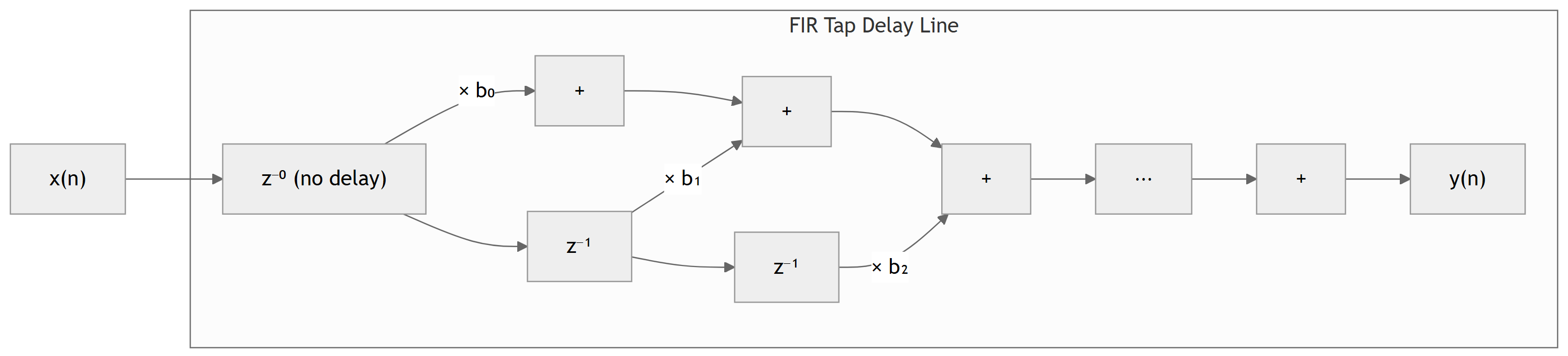
Visual: FIR Filter as a Tap Delay Line

Use this diagram to reinforce that FIR is just:

• Shift register (delays)
• Multipliers by coefficients
• Adders

Easy mapping to FPGA or DSP processor implementation.

7.2 Fourier Transform Design – Starting from an Ideal Filter

We begin with an ideal lowpass filter with normalized cutoff frequency \(\Omega_c\). Its ideal frequency response is:

\[ H(e^{j\Omega}) = \begin{cases} 1, & 0 \le |\Omega| \le \Omega_c, \\ 0, & \Omega_c \le |\Omega| \le \pi. \end{cases} \]

• \(\Omega\) is the normalized digital frequency in radians/sample.
• This is a brick-wall (perfect) lowpass filter on the unit circle.

FIG. 7.1 Frequency response of an ideal lowpass filter.

Remind:

• The DTFT is periodic in \(\Omega\) with period \(2\pi\).
• The magnitude response describes how each discrete-time sinusoid is scaled.

Make sure they understand that this filter is non-realizable directly (noncausal, infinite support), but it’s a good starting point.

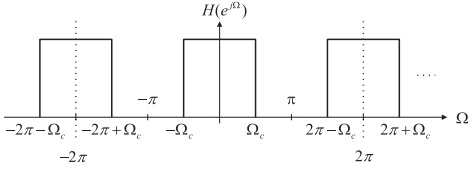
Ideal Lowpass – Periodic Extension

Because \(H(e^{j\Omega})\) is \(2\pi\)-periodic, we can extend it beyond \(-\pi\) to \(\pi\):

FIG. 7.2 Periodicity of the ideal lowpass frequency response.

Idea:

• View \(H(e^{j\Omega})\) as a periodic function of \(\Omega\).
• Then express it as a Fourier series in \(\Omega\).
• The Fourier series coefficients in \(\Omega\)-domain will turn out to be the impulse response \(h(n)\).

Frequency-Domain Fourier Series Representation

Write the periodic spectrum as a complex Fourier series in \(\Omega\):

\[ H(e^{j\Omega}) = \sum_{n=-\infty}^{\infty} c_n e^{-j \omega_0 n \Omega}. \]

Fourier series coefficients:

\[ c_n = \frac{1}{2\pi} \int_{-\pi}^{\pi} H(e^{j\Omega}) e^{j \omega_0 n \Omega} \, d\Omega. \]

For our case, the period is \(2\pi\), so:

\[ \omega_0 = \frac{2\pi}{2\pi} = 1. \]

So the series simplifies to:

\[ H(e^{j\Omega}) = \sum_{n=-\infty}^{\infty} c_n e^{-j n \Omega}. \]

Define \(h(n) = c_n\) ⇒

\[ H(e^{j\Omega}) = \sum_{n=-\infty}^{\infty} h(n) e^{-j n \Omega}. \]

and the corresponding “inverse” formula:

\[ h(n) = \frac{1}{2\pi} \int_{-\pi}^{\pi} H(e^{j\Omega}) e^{j n \Omega} \, d\Omega. \]

Note

This is just the DTFT pair: - \(H(e^{j\Omega}) \leftrightarrow h(n)\). - Except here, we are thinking of using it as a design formula to derive the ideal impulse response from the desired magnitude response.

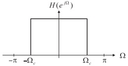
Ideal Lowpass – Desired (Infinite) Impulse Response

Apply the formula

\[ h(n) = \frac{1}{2\pi} \int_{-\pi}^{\pi} H(e^{j\Omega}) e^{j n \Omega} \, d\Omega \]

with \(H(e^{j\Omega}) = 1\) for \(|\Omega|\le \Omega_c\) and 0 otherwise.

For \(n = 0\):

\[ \begin{aligned} h(0) &= \frac{1}{2\pi} \int_{-\pi}^{\pi} H(e^{j\Omega})\, d\Omega \\ &= \frac{1}{2\pi} \int_{-\Omega_c}^{\Omega_c} 1 \, d\Omega \\ &= \frac{\Omega_c}{\pi}. \end{aligned} \]

For \(n \ne 0\):

\[ \begin{aligned} h(n) &= \frac{1}{2\pi} \int_{-\Omega_c}^{\Omega_c} e^{j n \Omega} \, d\Omega \\ &= \frac{1}{2\pi} \left[ \frac{e^{j n \Omega}}{j n} \right]_{-\Omega_c}^{\Omega_c} \\ &= \frac{1}{\pi n} \cdot \frac{e^{j n \Omega_c} - e^{-j n \Omega_c}}{2j} \\ &= \frac{\sin(\Omega_c n)}{\pi n}. \end{aligned} \]

So the ideal lowpass impulse response is:

\[ h(n) = \begin{cases} \dfrac{\Omega_c}{\pi}, & n = 0, \\ \dfrac{\sin(\Omega_c n)}{\pi n}, & n \neq 0. \end{cases} \]

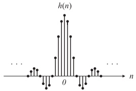
Ideal Lowpass Impulse Response Shape

FIG. 7.3 Impulse response of an ideal digital lowpass filter.

Observations:

• \(h(n)\) is infinite-length (exists for all integer \(n\)).
• Symmetric around \(n = 0\): \(h(n) = h(-n)\).
• Amplitude decays roughly like \(1/|n|\).

This is essentially a discrete-time sinc function:

\[ h(n) \propto \frac{\sin(\Omega_c n)}{n}. \]

Connect to continuous-time sinc used for ideal lowpass filter in analog and in sampling/reconstruction theory.

Mention that evenness of \(H(e^{j\Omega})\) (symmetry in frequency) leads to a real, even impulse response \(h(n)\).

From Ideal Infinite Impulse Response to FIR

The ideal impulse response is noncausal and infinite:

\[ H(z) = \sum_{n=-\infty}^{\infty} h(n) z^{-n} = \cdots + h(-2) z^{2} + h(-1) z^{1} + h(0) + h(1) z^{-1} + \cdots \]

Problems:

1. Infinite number of taps → impossible to implement exactly.
2. Contains positive powers of \(z\) ⇒ noncausal (depends on future inputs).

Practical FIR design steps:

1. Truncate \(h(n)\) to a finite index range \(-M \le n \le M\).

2. Use symmetry \(h(n) = h(-n)\) to form:

   \[ H(z) = h(M) z^{M} + \cdots + h(1) z^{1} + h(0) + h(1) z^{-1} + \cdots + h(M) z^{-M}. \]

3. Shift by \(M\) samples to make it causal:

   • Define \(b_n = h(n - M)\), for \(n = 0,1,\dots,2M\).

   • Then

     \[ H(z) = b_0 + b_1 z^{-1} + \cdots + b_{2M} z^{-2M}. \]

Important

Truncation + shift = basic FIR design by Fourier method.

But: abrupt truncation ⇒ Gibbs effect (ripples in passband and stopband). The window method is our fix.

Summary Table for Ideal FIR Impulse Responses

Table 7.1 (noncausal ideal coefficients \(h(n)\), \(-M \le n \le M\)):

Filter Type	Ideal Impulse Response \(h(n)\)
Lowpass	\(h(0) = \dfrac{\Omega_c}{\pi}\) and \(h(n) = \dfrac{\sin(\Omega_c n)}{n\pi},\; n\neq 0\)
Highpass	\(h(0) = \dfrac{\pi - \Omega_c}{\pi}\) and \(h(n) = -\dfrac{\sin(\Omega_c n)}{n\pi},\; n\neq 0\)
Bandpass	\(h(0) = \dfrac{\Omega_H - \Omega_L}{\pi}\) and \(h(n) = \dfrac{\sin(\Omega_H n)}{n\pi} - \dfrac{\sin(\Omega_L n)}{n\pi},\; n\neq 0\)
Bandstop	\(h(0) = \dfrac{\pi - \Omega_H + \Omega_L}{\pi}\) and \(h(n) = -\dfrac{\sin(\Omega_H n)}{n\pi} + \dfrac{\sin(\Omega_L n)}{n\pi},\; n\neq 0\)

Then make it causal by shifting: \(b_n = h(n-M)\).

Point out that all these formulas come from applying the inverse DTFT to the appropriate ideal magnitude response (rectangular in some band).

This table is central: highlight that design = choose type + choose band edges + choose M.

Example 7.2 – 3-Tap Lowpass by Fourier Design

Goal: Design a 3-tap (\(2M+1=3\) ⇒ \(M=1\)) lowpass FIR with:

• \(f_c = 800\) Hz, \(f_s = 8000\) Hz.

(a) Coefficients via Fourier method

Normalized cutoff:

\[ \Omega_c = 2\pi \frac{f_c}{f_s} = 2\pi \frac{800}{8000} = 0.2\pi \; \text{rad}. \]

From the lowpass formula:

\[ h(0) = \frac{\Omega_c}{\pi} = 0.2, \quad h(1) = \frac{\sin(0.2\pi)}{\pi} \approx 0.1871, \quad h(-1) = h(1) = 0.1871. \]

Shift by \(M=1\) to get causal coefficients:

\[ \begin{aligned} b_0 &= h(-1) = 0.1871, \\ b_1 &= h(0) = 0.2, \\ b_2 &= h(1) = 0.1871. \end{aligned} \]

Example 7.2 – Transfer Function and Difference Equation

2. Transfer function:

\[ H(z) = 0.1871 + 0.2 z^{-1} + 0.1871 z^{-2}. \]

Difference equation (inverse \(z\)-transform):

\[ y(n) = 0.1871 x(n) + 0.2 x(n-1) + 0.1871 x(n-2). \]

This is a symmetric 3-tap FIR lowpass filter.

Example 7.2 – Frequency Response and Linear Phase

3. Substitute \(z = e^{j\Omega}\):

\[ H(e^{j\Omega}) = 0.1871 + 0.2 e^{-j\Omega} + 0.1871 e^{-j2\Omega}. \]

Factor \(e^{-j\Omega}\):

\[ \begin{aligned} H(e^{j\Omega}) &= e^{-j\Omega} \left( 0.1871 e^{j\Omega} + 0.2 + 0.1871 e^{-j\Omega} \right) \\ &= e^{-j\Omega} \left( 0.2 + 0.3742 \cos\Omega \right). \end{aligned} \]

Magnitude and phase:

\[ |H(e^{j\Omega})| = \big|0.2 + 0.3742 \cos\Omega\big|, \]

\[ \angle H(e^{j\Omega}) = \begin{cases} -\Omega, & 0.2 + 0.3742 \cos\Omega > 0, \\ -\Omega + \pi, & 0.2 + 0.3742 \cos\Omega < 0. \end{cases} \]

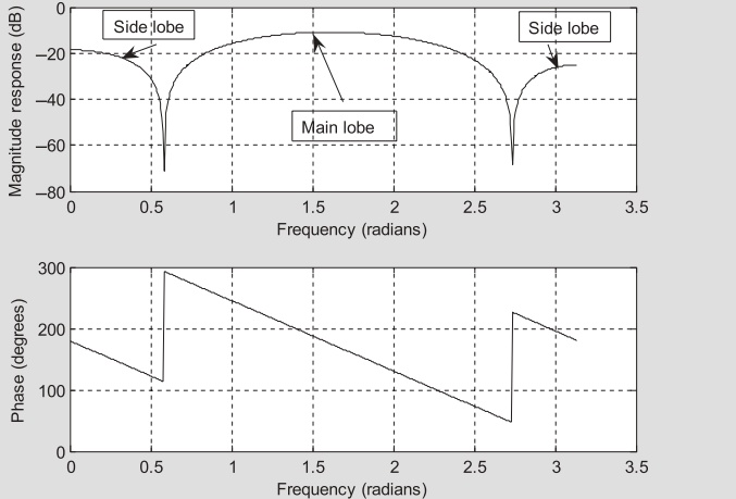
• Main slope of phase: \(-\Omega\) ⇒ linear phase with delay \(M=1\).
• Occasional \(\pi\) jumps when term in parentheses changes sign (sawtooth pattern).

Tip

For an FIR with symmetric coefficients and odd length \(2M+1\):

\[ \angle H(e^{j\Omega}) \approx -M \Omega \quad (\text{plus possible }180^\circ \text{ jumps}). \]

⇒ Constant group delay \(M\) samples for all passband frequencies.

Visual: 3-Tap vs 17-Tap Lowpass Filters

FIG. 7.5 Magnitude and phase responses of 3-tap (dash-dotted) and 17-tap (solid) lowpass FIR filters with \(\Omega_c = 0.2\pi\).

Observations:

1. 3-tap filter:
   • Wide transition band.
   • Significant ripples in passband and stopband.
2. 17-tap filter (\(M=8\)):
   • Sharper transition.
   • Still has ripples (Gibbs effect), but narrower transition band.

Trade-off: more taps ⇒ better frequency selectivity, but:

• More computations per sample.
• Larger delay (here, \(M=8\) samples).

Gibbs Effect – Why Ripples Appear

The passband and stopband ripples in ideal-based FIR design come from:

• Abrupt truncation of the infinite impulse response.

Analogy:

• Truncating a continuous-time sinc (multiplying by a rectangular window) produces ripples in frequency.

In our discrete-time design:

• Multiplying the ideal infinite \(h(n)\) by a finite-length rectangular window in time ⇒ convolution with sinc-like main/side lobes in frequency ⇒ ripples (Gibbs).

We will reduce these ripples by using smoother windows (Hanning, Hamming, Blackman, etc.) instead of the abrupt rectangular window.

Linear Phase and Waveform Preservation

Because the FIR coefficients are symmetric, the filter has linear phase:

\[ \angle H(e^{j\Omega}) \approx -M\Omega. \]

If input is a sinusoid \(x(n) = A \sin(\Omega n)\), the steady-state output is:

\[ y(n) = A |H(e^{j\Omega})| \sin\big(\Omega(n - M)\big). \]

• Same frequency.
• Same waveform shape.
• Only delayed by \(M\) samples and scaled in amplitude.

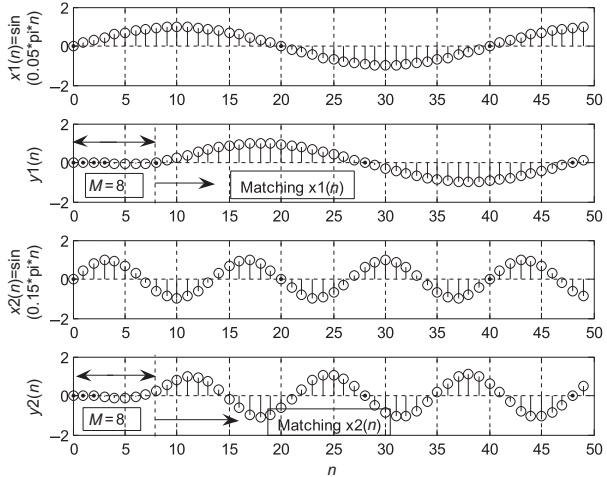
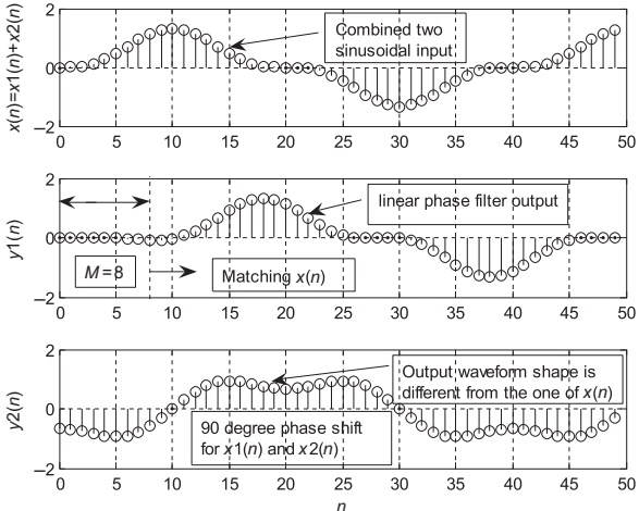
For a sum of sinusoids within the passband, all components get same delay ⇒ waveform shape is preserved ⇒ no phase distortion.

FIG. 7.6: Input and output sinusoidal signals, showing constant delay (linear phase).

What if Phase Is Nonlinear?

Consider input (sum of two sinusoids):

\[ x(n) = \sin(0.05\pi n) u(n) - \frac{1}{3} \sin(0.15\pi n) u(n). \]

1. Linear phase filter (delay 8 samples):

   \[ y_1(n) = \sin\big(0.05\pi(n-8)\big) - \frac{1}{3}\sin\big(0.15\pi(n-8)\big). \]

   • Entire signal looks like delayed copy of \(x(n)\).

2. Nonlinear phase filter with \(90^\circ\) phase shift at both frequencies:

   \[ y_2(n) = \sin(0.05\pi n - \pi/2) - \frac{1}{3} \sin(0.15\pi n - \pi/2). \]

   • Delay depends on frequency (10 samples vs \(10/3\) samples).
   • Waveform shape changes: phase distortion.

FIG. 7.7 Comparison of linear and nonlinear phase responses.

In audio: nonlinear phase can make transients smeared or “hollow” sounding ⇒ FIR linear-phase filters are desirable.

Example 7.3 – 5-Tap Bandpass Filter

Specs:

• \(f_L = 2000\) Hz, \(f_H = 2400\) Hz, \(f_s = 8000\) Hz.
• 5 taps ⇒ \(2M+1 = 5\) ⇒ \(M = 2\).

Normalized edges:

\[ \Omega_L = 2\pi \frac{2000}{8000} = 0.5\pi, \quad \Omega_H = 2\pi \frac{2400}{8000} = 0.6\pi. \]

Ideal bandpass impulse (noncausal):

\[ h(0) = \frac{\Omega_H - \Omega_L}{\pi} = 0.1. \]

\[ h(1) = \frac{\sin(0.6\pi)}{\pi} - \frac{\sin(0.5\pi)}{\pi} \approx -0.01558, \]

\[ h(2) = \frac{\sin(1.2\pi)}{2\pi} - \frac{\sin(\pi)}{2\pi} \approx -0.09355, \]

with symmetry:

\[ h(-1)=h(1),\quad h(-2)=h(2). \]

Shift by \(M=2\):

\[ b_0 = b_4 = -0.09355, \quad b_1 = b_3 = -0.01558, \quad b_2 = 0.1. \]

Transfer function:

\[ H(z) = -0.09355 - 0.01558 z^{-1} + 0.1 z^{-2} - 0.01558 z^{-3} - 0.09355 z^{-4}. \]

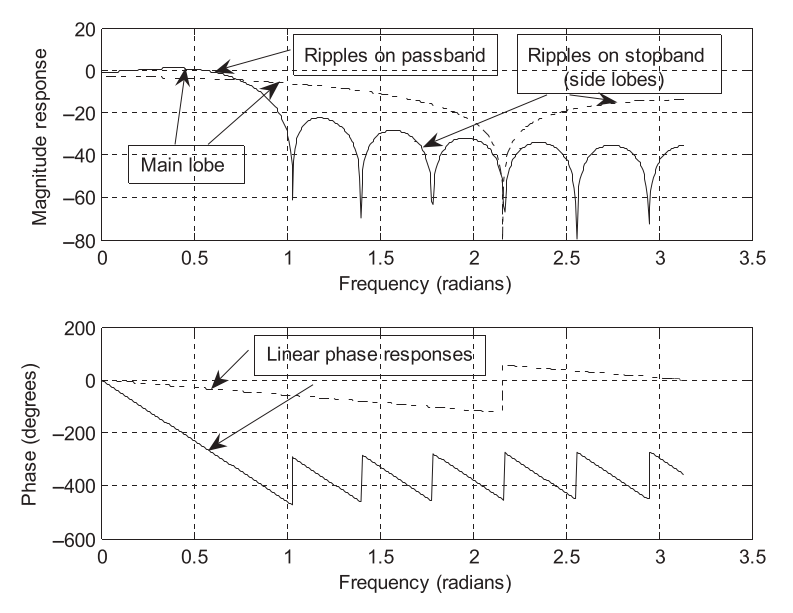
Example 7.3 – Observing Gibbs in Bandpass

MATLAB frequency response (Program 7.1) gives:

FIG. 7.8 Frequency responses for Example 7.3.

Observations:

• Passband peak is ~\(-10\) dB instead of 0 dB.
• Stopband side lobes swing between roughly -18 and -70 dB (lower) and -25 and -68 dB (upper).
• This is again Gibbs oscillation, due to abrupt truncation.

Fix: Window the impulse response instead of raw truncation.

7.3 Window Method – Motivation

We know:

• Truncating the ideal, infinite \(h(n)\) with a rectangular window (just cutting off) gives Gibbs ripples.

Idea:

• Replace sharp truncation with smoother weighting that tapers to zero at the ends.

Mathematically:

\[ h_w(n) = h(n)\, w(n), \]

where \(w(n)\) is a window function, nonzero for \(-M \le n \le M\), symmetric around 0.

Effect in frequency:

• Convolution of ideal response with window’s spectrum.
• Tapered windows reduce side lobes (ripples) but broaden main lobe (wider transition).

Common Window Functions

1. Rectangular:

\[ w_{\text{rec}}(n) = 1,\quad -M \le n \le M. \]

2. Triangular (Bartlett):

\[ w_{\text{tri}}(n) = 1 - \frac{|n|}{M},\quad -M \le n \le M. \]

3. Hanning:

\[ w_{\text{han}}(n) = 0.5 + 0.5\cos\left(\frac{\pi n}{M}\right),\quad -M \le n \le M. \]

4. Hamming:

\[ w_{\text{ham}}(n) = 0.54 + 0.46\cos\left(\frac{\pi n}{M}\right),\quad -M \le n \le M. \]

5. Blackman:

\[ w_{\text{black}}(n) = 0.42 + 0.5\cos\left(\frac{\pi n}{M}\right) + 0.08\cos\left(\frac{2\pi n}{M}\right),\quad -M \le n \le M. \]

FIG. 7.9 Shapes of window functions for \(2M+1=81\).

• Rectangular: abrupt edges.
• Others: smooth taper to zero at ends.

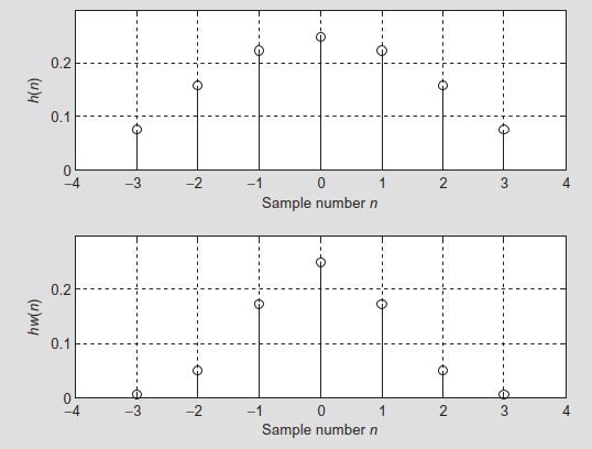
Example 7.4 – Applying Hamming Window to FIR Coefficients

Given noncausal symmetric coefficients (ideal lowpass):

\[ h(0)=0.25,\; h(\pm1)=0.22508,\; h(\pm2)=0.15915,\; h(\pm3)=0.07503. \]

Use Hamming window with \(M=3\):

Window values:

\[ \begin{aligned} w_{\text{ham}}(0) &= 0.54 + 0.46 \cos(0) = 1.0, \\ w_{\text{ham}}(\pm 1) &= 0.77, \\ w_{\text{ham}}(\pm 2) &= 0.31, \\ w_{\text{ham}}(\pm 3) &= 0.08. \end{aligned} \]

Windowed coefficients:

\[ \begin{aligned} h_w(0) &= 0.25 \times 1 = 0.25, \\ h_w(\pm1) &= 0.22508 \times 0.77 \approx 0.17331, \\ h_w(\pm2) &= 0.15915 \times 0.31 \approx 0.04934, \\ h_w(\pm3) &= 0.07503 \times 0.08 \approx 0.00600. \end{aligned} \]

FIG. 7.10 Ideal vs windowed coefficients \(h(n)\) and \(h_w(n)\).

Observation: coefficients are smoothly tapered toward zero ⇒ reduced Gibbs ripples.

FIR Design via Windowing – 3-Step Recipe

1. Design ideal truncated impulse response \(h(n)\):

   • Use formulas in Table 7.1.
   • Choose filter type (lowpass, highpass, bandpass, bandstop).
   • Choose \(M\) (length \(2M+1\)).

2. Apply window:

   \[ h_w(n) = h(n)\, w(n),\quad -M \le n \le M. \]

   • Choose \(w(n)\): rectangular, Hanning, Hamming, Blackman, etc.

3. Make it causal by shifting \(M\) samples:

   \[ b_n = h_w(n - M),\quad n = 0, 1, \dots, 2M. \]

   • Implement FIR with coefficients \(b_n\).

Example 7.5 – 3-Tap Lowpass with Hamming Window

Same spec as Example 7.2:

• \(f_c = 800\) Hz, \(f_s = 8000\) Hz ⇒ \(\Omega_c = 0.2\pi\).
• \(2M+1 = 3\) ⇒ \(M = 1\).

Ideal coefficients (from Example 7.2):

\[ h(0) = 0.2,\quad h(\pm1) = 0.1871. \]

Hamming window (for \(M=1\)):

\[ w_{\text{ham}}(0) = 1,\quad w_{\text{ham}}(\pm1) = 0.08. \]

Windowed noncausal coefficients:

\[ \begin{aligned} h_w(0) &= 0.2 \times 1 = 0.2, \\ h_w(\pm 1) &= 0.1871 \times 0.08 \approx 0.01497. \end{aligned} \]

Shift by \(M=1\):

\[ b_0 = b_2 = 0.01497,\quad b_1 = 0.2. \]

Transfer function:

\[ H(z) = 0.01497 + 0.2 z^{-1} + 0.01497 z^{-2}. \]

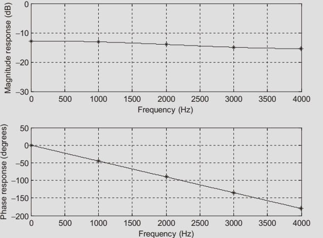
Example 7.5 – Frequency Response

Frequency response:

\[ H(e^{j\Omega}) = e^{-j\Omega}\big(0.2 + 0.02994\cos\Omega\big). \]

Magnitude:

\[ |H(e^{j\Omega})| = \big|0.2 + 0.02994\cos\Omega\big|. \]

Phase:

\[ \angle H(e^{j\Omega})= \begin{cases} -\Omega, & 0.2 + 0.02994\cos\Omega > 0, \\ -\Omega + \pi, & 0.2 + 0.02994\cos\Omega < 0. \end{cases} \]

Sample values (Table 7.4) show slightly reduced peak magnitude and less ripple compared to the unwindowed case.

FIG. 7.11 Frequency responses in Example 7.5.

Example 7.6 – 5-Tap Bandstop with Hamming Window

Specs:

• Bandreject (notch) from 2000–2400 Hz.
• \(f_s = 8000\) Hz.
• 5 taps ⇒ \(M=2\).

Ideal bandstop \(h(n)\) (Table 7.1):

\[ h(0) = \frac{\pi - \Omega_H + \Omega_L}{\pi} = 0.9, \]

\[ h(1) \approx 0.01558, \quad h(2) \approx 0.09355, \quad h(-1)=h(1),\; h(-2)=h(2). \]

Hamming window (\(M=2\)):

\[ w_{\text{ham}}(0) = 1,\quad w_{\text{ham}}(\pm1)=0.54,\quad w_{\text{ham}}(\pm2)=0.08. \]

Windowed coefficients:

\[ \begin{aligned} h_w(0) &= 0.9, \\ h_w(\pm1) &= 0.01558\times0.54\approx0.00841, \\ h_w(\pm2) &= 0.09355\times0.08\approx0.00748. \end{aligned} \]

Shift by \(M=2\):

\[ b_0 = b_4 = 0.00748,\quad b_1 = b_3 = 0.00841,\quad b_2 = 0.9. \]

Transfer function:

\[ H(z) = 0.00748 + 0.00841 z^{-1} + 0.9 z^{-2} + 0.00841 z^{-3} + 0.00748 z^{-4}. \]

MATLAB Helper Function: firwd

For larger designs, we let MATLAB do the heavy lifting. Custom function:

B = firwd(N, Ftype, WnL, WnH, Wtype)

• N: number of taps (must be odd).
• Ftype:
  • 1 = lowpass
  • 2 = highpass
  • 3 = bandpass
  • 4 = bandreject
• WnL, WnH: lower and upper cutoff frequencies (in radians).
  • For lowpass: set WnH = 0, use WnL = Ω_c.
  • For highpass: set WnL = 0, use WnH = Ω_c.

• Wtype:
  • 1 = rectangular
  • 2 = triangular
  • 3 = Hanning
  • 4 = Hamming
  • 5 = Blackman

This function internally:

1. Generates ideal \(h(n)\) using formulas like Table 7.1.
2. Multiplies by chosen window \(w(n)\).
3. Shifts to produce causal coefficients \(B\).

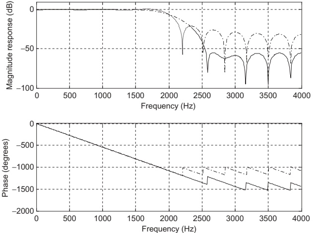
Example 7.7 – 25-Tap Lowpass: Rectangular vs Hamming

Specs:

• Lowpass, \(f_c = 2000\) Hz, \(f_s = 8000\) Hz.
• 25 taps ⇒ \(M=12\).
• \(\Omega_c = 0.5\pi\).

Use firwd twice:

• Rectangular window (Wtype=1).
• Hamming window (Wtype=4).

Magnitude responses:

FIG. 7.12 Rectangular (dash-dotted) vs Hamming (solid) window lowpass responses.

Observations:

• Rectangular: narrower transition but higher side lobes (~-21 dB).
• Hamming: slightly wider transition but lower side lobes (~-53 dB).

Coefficients listed in Table 7.6.

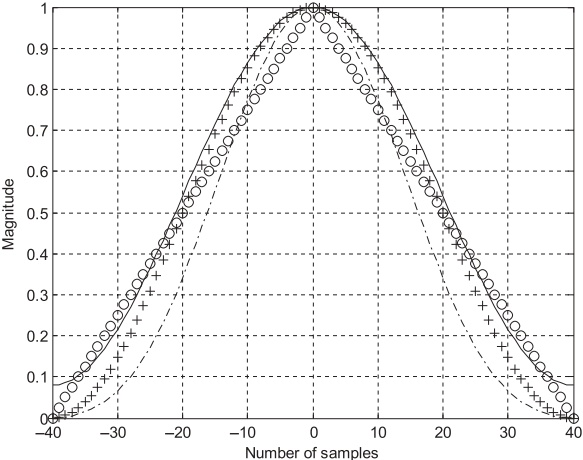
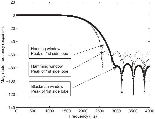
Comparing Hanning, Hamming, Blackman

For the same lowpass spec (25 taps, \(f_c=2000\) Hz):

FIG. 7.13 Magnitude responses with different windows: Hanning vs Hamming vs Blackman

Qualitative summary:

• Hanning: medium main-lobe width, moderate side lobes (~-44 dB).
• Hamming: similar main-lobe width, lower side lobes (~-53 dB).
• Blackman: wider main lobe, very low side lobes (~-74 dB).

Trade-off:

• Better stopband attenuation ⇒ more main-lobe widening (worse transition).

Window Performance and Length Estimation (Table 7.7)

For normalized transition width

\[ \Delta f = \frac{|f_{\text{stop}} - f_{\text{pass}}|}{f_s}, \]

approximate length for each window:

Window	\(w(n)\)	Length \(N\)	Passband Ripple (dB)	Stopband Atten (dB)
Rectangular	\(1\)	\(N \approx \dfrac{0.9}{\Delta f}\)	0.7416	21
Hanning	\(0.5+0.5\cos(\pi n/M)\)	\(N \approx \dfrac{3.1}{\Delta f}\)	0.0546	44
Hamming	\(0.54+0.46\cos(\pi n/M)\)	\(N \approx \dfrac{3.3}{\Delta f}\)	0.0194	53
Blackman	\(0.42+0.5\cos(\pi n/M)+0.08\cos(2\pi n/M)\)	\(N \approx \dfrac{5.5}{\Delta f}\)	0.0017	74

Design cutoff frequency:

\[ f_c = \frac{f_{\text{pass}} + f_{\text{stop}}}{2}. \]

Tip

Design recipe from specs:

1. From desired passband ripple and stopband attenuation, pick a window.
2. Compute \(\Delta f\) from the band edges.
3. Use table formula to estimate \(N\), then round up to next odd integer.
4. Compute \(f_c\) (lowpass/highpass) or \(f_L, f_H\) (band filters).
5. Use Fourier + window method (or firwd) to get coefficients.

Example 7.8 – Lowpass Length from Specs

Specs:

• Passband: 0–1850 Hz.
• Stopband: 2150–4000 Hz.
• Stopband attenuation: 20 dB.
• Passband ripple: 1 dB.
• \(f_s = 8000\) Hz.

Compute normalized transition width:

\[ \Delta f = \frac{|2150 - 1850|}{8000} = 0.0375. \]

Window choice:

• Rectangular gives ~0.74 dB ripple and 21 dB stopband attenuation ⇒ meets the requirements (1 dB ripple, 20 dB attenuation).

Length estimate:

\[ N = \frac{0.9}{\Delta f} = \frac{0.9}{0.0375} \approx 24. \]

Take odd \(N=25\).

Design cutoff frequency:

\[ f_c = \frac{1850 + 2150}{2} = 2000 \; \text{Hz}. \]

This is exactly the lowpass designed in Example 7.7.

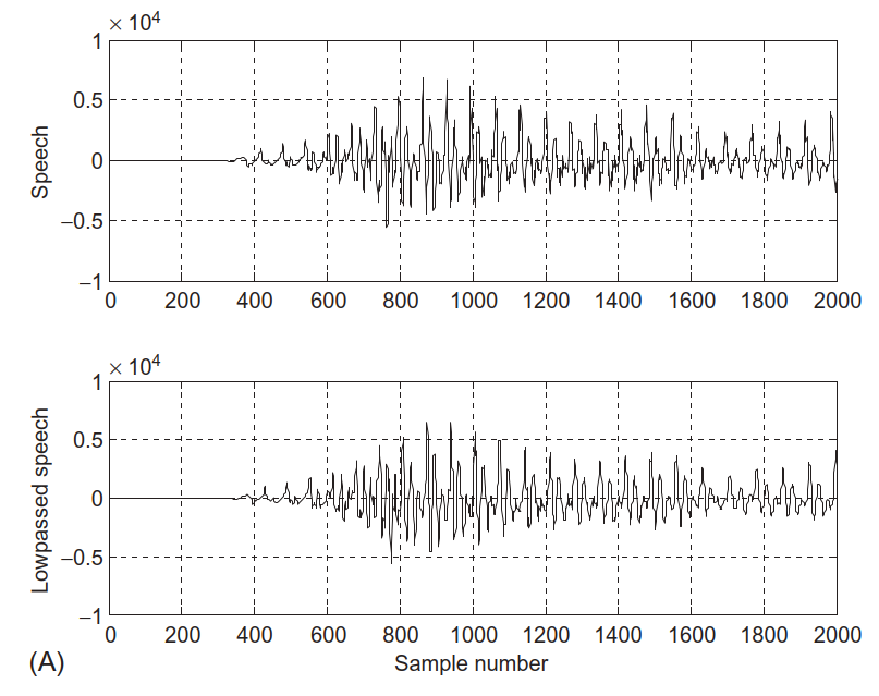
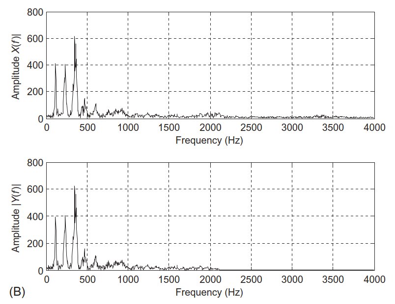
Example 7.8 – Effect on Speech

Apply this lowpass FIR to speech sampled at 8 kHz:

FIG. 7.15(A) Original speech vs lowpass filtered speech.

FIG. 7.15(B) Spectral comparison: high-frequency content beyond 2 kHz is removed.

Perceptually:

• Filtered speech sounds “muffled” because we removed higher harmonics and fricative energy.

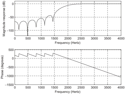
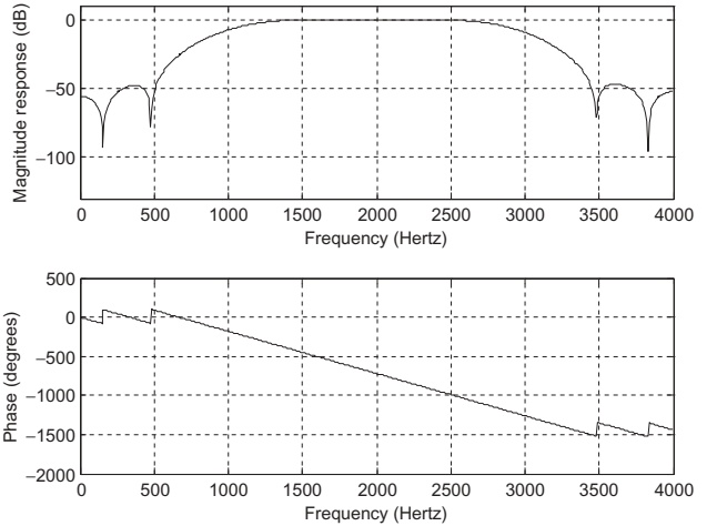
Example 7.9 – Highpass Filter from Specs

Specs:

• Stopband: 0–1500 Hz.
• Passband: 2500–4000 Hz.
• Stopband attenuation: 40 dB.
• Passband ripple: 0.1 dB.
• \(f_s = 8000\) Hz.

Transition width:

\[ \Delta f = \frac{|2500 - 1500|}{8000} = 0.125. \]

From Table 7.7:

• Need stopband ∼ 40 dB and small ripple ⇒ Hanning (≈44 dB, 0.0546 dB ripple) is acceptable.

Length estimate:

\[ N = \frac{3.1}{0.125} = 24.8 \Rightarrow N=25. \]

Cutoff frequency:

\[ f_c = \frac{1500+2500}{2} = 2000 \; \text{Hz}, \quad \Omega_c = 0.5\pi. \]

Use firwd(25, 2, 0, 0.5*pi, 3) to generate highpass coefficients.

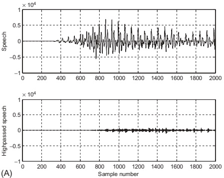
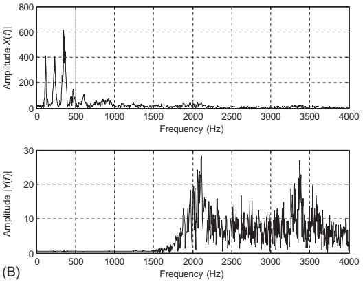
Example 7.9 – Effect on Speech

Frequency response:

FIG. 7.16 Highpass FIR designed with Hanning window.

Apply to speech:

FIG. 7.17(A) Original vs highpass filtered speech.h

FIG. 7.17(B) Frequencies below 1.5 kHz are removed.

Perceptually:

• Speech sounds “crisp” or “thin”, emphasizing sibilants and consonant noise.

Example 7.10 – Bandpass Design from Specs

Specs:

• Lower stopband: 0–500 Hz.
• Passband: 1600–2300 Hz.
• Upper stopband: 3500–4000 Hz.
• Stopband attenuation: 50 dB.
• Passband ripple: 0.05 dB.
• \(f_s = 8000\) Hz.

Compute transition widths:

\[ \Delta f_1 = \frac{1600-500}{8000} = 0.1375, \quad \Delta f_2 = \frac{3500-2300}{8000} = 0.15. \]

Using Hamming window (≈53 dB stopband, 0.0194 dB ripple):

\[ N_1 = \frac{3.3}{0.1375} \approx 24,\quad N_2 = \frac{3.3}{0.15} \approx 22. \]

Choose \(N=25\).

Cutoff frequencies for ideal bandpass:

\[ f_L = \frac{1600+500}{2} = 1050\; \text{Hz},\quad f_H = \frac{3500+2300}{2} = 2900\; \text{Hz}. \]

Normalized:

\[ \Omega_L = 0.2625\pi,\quad \Omega_H = 0.725\pi. \]

Use firwd(25, 3, Ω_L, Ω_H, 4) to generate Hamming-windowed bandpass FIR.

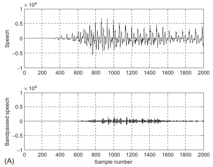
Example 7.10 – Bandpass on Speech

Frequency response:

FIG. 7.18 Bandpass response via Hamming window.

Coefficients in Table 7.9.

Filtering speech:

FIG. 7.19(A) Original vs bandpass filtered speech.

FIG. 7.19(B) Only midband frequencies in passband are preserved.

Example 7.11 – Bandstop Design from Specs

Specs:

• Lower cutoff: 1250 Hz.
• Lower transition width: 1500 Hz.
• Upper cutoff: 2850 Hz.
• Upper transition width: 1300 Hz.
• Stopband attenuation: 60 dB.
• Passband ripple: 0.02 dB.
• \(f_s = 8000\) Hz.

Transition widths:

\[ \Delta f_1 = \frac{1500}{8000} = 0.1875,\quad \Delta f_2 = \frac{1300}{8000} = 0.1625. \]

Need ≈60 dB attenuation ⇒ Blackman window (~74 dB).

Lengths:

\[ N_1 = \frac{5.5}{0.1875} \approx 29.3,\quad N_2 = \frac{5.5}{0.1625} \approx 33.8. \]

Choose odd \(N=35\).

Cutoff frequencies:

\[ \Omega_L = 2\pi\frac{1250}{8000} = 0.3125\pi,\quad \Omega_H = 2\pi\frac{2850}{8000} = 0.7125\pi. \]

Use firwd(35, 4, Ω_L, Ω_H, 5) to get bandstop FIR.

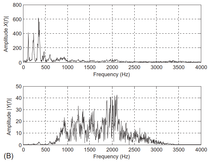
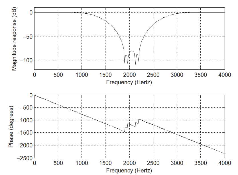
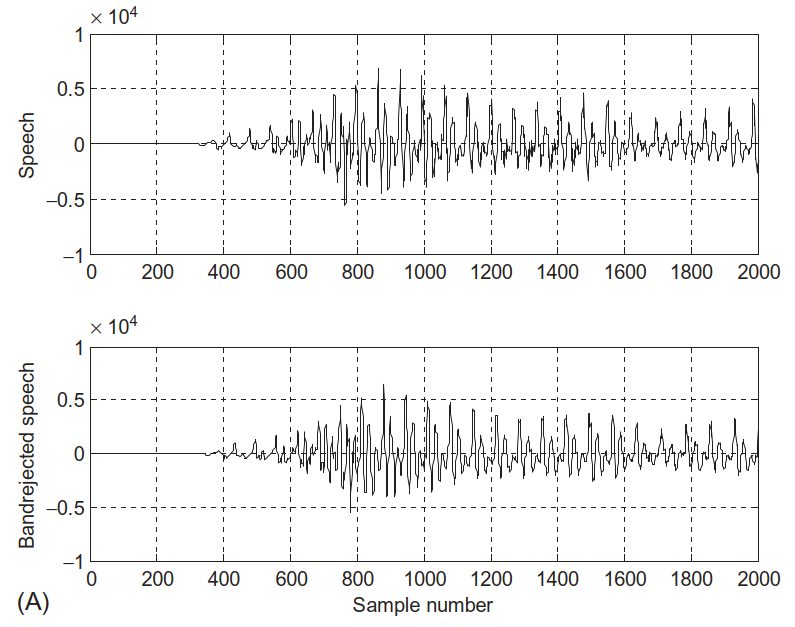
Example 7.11 – Bandstop on Speech

Frequency response:

FIG. 7.20 Bandstop FIR with Blackman window.

Coefficients in Table 7.10.

Filtering speech:

FIG. 7.21(A) Original vs bandstop filtered speech.

FIG. 7.21(B) Frequencies in the stop band (≈2000–2200 Hz) are strongly attenuated.

Use case: removing a narrowband interference (like a whistle) from speech.

In-Class Practice – Designing a Simple FIR

Problem:

Design a 7-tap lowpass FIR filter (\(N=7\), so \(M=3\)) with:

• \(f_c = 1000\) Hz, \(f_s = 8000\) Hz.
• Use the Hanning window.

Tasks:

1. Compute \(\Omega_c\).
2. Use Table 7.1 to compute noncausal ideal \(h(n)\), \(-3 \le n \le 3\).
3. Compute Hanning window \(w_{\text{han}}(n)\), \(-3 \le n \le 3\).
4. Compute \(h_w(n) = h(n) w(n)\).
5. Shift by \(M=3\) to find causal \(b_0,\dots,b_6\).

Work through one or two coefficients with the class, then let them complete in pairs.

Optionally, show how to verify frequency response using MATLAB or Python.

Key Takeaways – Conceptual

1. FIR format:
   • \(y(n) = \sum b_i x(n-i)\),
   • \(H(z) = \sum b_i z^{-i}\).
   • Always BIBO stable, easy to implement as tap delay line.
2. Fourier design method:
   • Start from ideal frequency response \(H_d(e^{j\Omega})\).
   • Use inverse DTFT to find ideal \(h_d(n)\).
   • Truncate and shift to get practical FIR.
3. Gibbs effect:
   • Abrupt truncation (rectangular window) causes ripples in passband/stopband.
4. Linear phase:
   • Symmetric FIR coefficients (odd length) ⇒ \(\angle H(e^{j\Omega})\) is linear in \(\Omega\).
   • All passband components delayed by same number of samples ⇒ no phase distortion.

Key Takeaways – Window Method and Design Rules

5. Window method:

   • \(h_w(n) = h_d(n)\, w(n)\).
   • Smoother windows (Hanning, Hamming, Blackman) reduce ripple (side lobes) but enlarge transition width (main lobe).

6. Window choices (rough performance):

   • Rectangular: short \(N\), poor attenuation (~21 dB).
   • Hanning: moderate \(N\), ~44 dB attenuation.
   • Hamming: moderate \(N\), ~53 dB attenuation (good general choice).
   • Blackman: long \(N\), ~74 dB attenuation (for tight specs).

7. Filter length from specs:

   • Compute normalized transition width \(\Delta f\).
   • Choose window based on required ripple & attenuation.
   • Use table: \(N \approx \text{constant}/\Delta f\).
   • Make \(N\) odd for symmetric, linear-phase FIR.

8. Real-world ECE:

   • Designed filters applied to speech to control timbre and remove noise.
   • Same ideas apply to OFDM subcarrier shaping, channel equalization, biomedical signal filtering, etc.

Formula Summary

FIR structure:

\[ y(n) = \sum_{i=0}^{K} b_i x(n-i),\quad H(z) = \sum_{i=0}^{K} b_i z^{-i}. \]

Frequency response (DTFT of impulse response):

\[ H(e^{j\Omega}) = \sum_{n=-\infty}^{\infty} h(n) e^{-jn\Omega}. \]

Inverse DTFT (design equation):

\[ h(n) = \frac{1}{2\pi}\int_{-\pi}^{\pi} H(e^{j\Omega}) e^{jn\Omega} \, d\Omega. \]

Ideal lowpass impulse response:

\[ h(n) = \begin{cases} \frac{\Omega_c}{\pi}, & n=0, \\ \frac{\sin(\Omega_c n)}{\pi n}, & n\neq 0. \end{cases} \]

Other ideal FIRs (noncausal):

Lowpass:

\[ h(n) = \frac{\Omega_c}{\pi} \text{ for } n=0;\quad h(n) = \frac{\sin(\Omega_c n)}{n\pi} \text{ for } n\neq 0. \]

Highpass:

\[ h(0) = \frac{\pi - \Omega_c}{\pi};\quad h(n) = -\frac{\sin(\Omega_c n)}{n\pi},\; n\neq 0. \]

Bandpass:

\[ h(0) = \frac{\Omega_H - \Omega_L}{\pi};\quad h(n) = \frac{\sin(\Omega_H n)}{n\pi} - \frac{\sin(\Omega_L n)}{n\pi},\; n\neq 0. \]

Bandstop:

\[ h(0) = \frac{\pi - \Omega_H + \Omega_L}{\pi};\quad h(n) = -\frac{\sin(\Omega_H n)}{n\pi} + \frac{\sin(\Omega_L n)}{n\pi},\; n\neq 0. \]

Windowing:

\[ h_w(n) = h(n) w(n),\quad -M \le n \le M. \]

Causal coefficients:

\[ b_n = h_w(n-M),\quad n=0,1,\dots,2M. \]

Linear phase (symmetric FIR, odd length):

\[ \angle H(e^{j\Omega}) = -M\Omega \; (+ \text{optional } \pi \text{ jumps}). \]

Transition width and length (example for Hamming):

\[ \Delta f = \frac{|f_{\text{stop}} - f_{\text{pass}}|}{f_s},\quad N \approx \frac{3.3}{\Delta f}. \]

\[ f_c = \frac{f_{\text{pass}} + f_{\text{stop}}}{2}. \]

FIR Filter Design – Interactive Deck

How to Use This Interactive Deck

• All code runs in your browser using Pyodide (Python in WebAssembly).
• You can:
  • Edit and run Python code ({pyodide} blocks).
  • Use sliders and controls ({ojs} blocks) to change parameters.
  • See FIR impulse and frequency responses update live with Plotly.

Try to:

• Change cutoff frequencies.
• Change filter length (N).
• Change window type.
• Observe the effects on ripples, transition width, and phase.

Explain to students that this deck is for exploration. Encourage them to “break” things: choose extreme parameter values and see what happens.

Make sure the environment is set up with Pyodide, Plotly, and OJS in Quarto. Usually this just works in the browser for Quarto Reveal presentations.

Warm-Up: Evaluate a Simple FIR Filter in Python

Task: Change the coefficients and input samples and re-run the code.

Try:

• Change b to [1/3, 1/3, 1/3] → moving average lowpass.
• Change x to a step: [0, 0, 1, 1, 1, 1].

After they run, ask:

• Is this filter “smoothing” or “sharpening”?
• Compare shape of y to x.

Reinforce the implementation structure: multiply–accumulate over past inputs only.

Interactive: Impulse Response of an Ideal Lowpass (Analytical)

We know the ideal lowpass impulse response is

\[ h(n) = \begin{cases} \Omega_c / \pi, & n = 0, \\ \sin(\Omega_c n) / (\pi n), & n \neq 0. \end{cases} \]

Use the sliders to see how \(\Omega_c\) and truncation index \(M\) affect \(h(n)\).

viewof oc = Inputs.range([0.1, 0.9], {step: 0.05, label: "Normalized cutoff Ω_c / π"})
viewof M  = Inputs.range([3, 40], {step: 1, label: "Truncation index M (half-length)"} )

Ask:

• What happens to the shape as M increases?
• Does h(n) look more “sinc-like” for large M?

Point out symmetry: \(h(n) = h(-n)\).

Interactive: From Ideal Noncausal \(h(n)\) to Causal \(b_n\)

We shift the impulse response by \(M\) samples to get a causal FIR:

\[ b_n = h(n - M), \quad n = 0,\dots,2M. \]

Interactively see the effect of the shift.

viewof M_shift = Inputs.range([3, 20], {step: 1, label: "M (shift, and half-length)"})

Point out:

• The shape is the same, only shifted right.
• The causal version starts at n=0; all negative-time samples are moved to positive n.

Interactive: Magnitude Response of an Ideal-Truncated Lowpass

Now we compute the DTFT of truncated \(h(n)\) and plot \(|H(e^{j\Omega})|\).

viewof oc2 = Inputs.range([0.1, 0.9], {step: 0.05, label: "Normalized cutoff Ω_c / π"})
viewof M2  = Inputs.range([5, 60], {step: 1, label: "M (truncation index)"} )

Explore:

• Increase \(M\) ⇒ transition narrows, side lobes get closer together.
• Observe Gibbs ripples near the cutoff.

Interactive: Add a Window – Compare Rectangular vs Hamming

We now apply a window to \(h(n)\):

\[ h_w(n) = h(n) w(n). \]

Compare rectangular and Hamming windows.

viewof oc3 = Inputs.range([0.1, 0.9], {step: 0.05, label: "Normalized cutoff Ω_c / π"})
viewof M3  = Inputs.range([5, 60], {step: 1, label: "M (half-length)"} )
viewof wtype = Inputs.select(
  ["Rectangular", "Hamming", "Both"],
  {label: "Window type", value: "Both"}
)

Observe:

• Rectangular: sharper transition, higher side lobes.
• Hamming: slightly wider main lobe, much lower side lobes.

Interactive: Window Choices – Hanning vs Hamming vs Blackman

Play with different windows and see main-lobe / side-lobe trade-offs.

viewof oc4 = Inputs.range([0.1, 0.9], {step: 0.05, label: "Normalized cutoff Ω_c / π"})
viewof M4  = Inputs.range([10, 80], {step: 2, label: "M (half-length)"} )
viewof wmulti = Inputs.checkbox(
  ["Rectangular", "Hanning", "Hamming", "Blackman"],
  {label: "Windows to plot", value: ["Rectangular", "Hanning", "Hamming", "Blackman"]}
)

Try:

• Compare Blackman vs Hamming: note much lower side lobes but wider transition.
• Turn windows on/off to see differences clearly.

Interactive: Length Estimation from Specs (Table 7.7)

Use the rules of thumb to estimate \(N\) from transition width \(\Delta f\).

viewof df = Inputs.range([0.01, 0.3], {step: 0.005, label: "Normalized transition width Δf"})
viewof win_choice = Inputs.select(
  ["Rectangular", "Hanning", "Hamming", "Blackman"],
  {label: "Window type", value: "Hamming"}
)

Experiment:

• Narrower (f) ⇒ larger (N).
• Different windows need different lengths to achieve similar transition widths.

Interactive: Build a Lowpass Filter to Spec (Full Workflow)

Let’s approximate a lowpass design with:

• Passband edge \(f_{pass}\).
• Stopband edge \(f_{stop}\).
• Sampling rate \(f_s = 8000\) Hz (fixed).
• Choose window type.

viewof fpass = Inputs.range([500, 3500], {step: 100, label: "Passband edge f_pass (Hz)", value: 1800})
viewof fstop = Inputs.range([600, 3900], {step: 100, label: "Stopband edge f_stop (Hz)", value: 2200})
viewof wdesign = Inputs.select(
  ["Rectangular", "Hanning", "Hamming", "Blackman"],
  {label: "Window type", value: "Hamming"}
)

Challenge:

• Try to match the spec from Example 7.8 (0–1850 Hz passband, 2150–4000 Hz stopband).
• Compare your chosen window and N to the textbook’s.

Interactive: Time-Domain Filtering of a Sinusoid Sum

Test the linear phase property of a symmetric FIR on a sum of sinusoids.

viewof f1 = Inputs.range([200, 1500], {step: 50, label: "Sinusoid 1 frequency f1 (Hz)", value: 400})
viewof f2 = Inputs.range([500, 3000], {step: 50, label: "Sinusoid 2 frequency f2 (Hz)", value: 1200})
viewof Nd = Inputs.range([5, 41], {step: 2, label: "Filter length N (odd)", value: 17})
viewof ocd = Inputs.range([0.1, 0.9], {step: 0.05, label: "Normalized cutoff Ω_c / π for lowpass", value: 0.4})

Explore:

• Adjust \(f_1\) and \(f_2\) to be both below cutoff, both above, or one below and one above.
• Watch how the waveform shape and delay change.

Summary & Next Steps

In this interactive deck you:

• Implemented FIR filtering in Python.
• Built ideal lowpass impulse responses and made them causal.
• Visualized the Gibbs effect with finite-length truncation.
• Applied different windows and saw main-lobe / side-lobe trade-offs.
• Used spec-based formulas to estimate FIR length and design complete filters.
• Observed linear-phase behavior in the time domain.

Suggested follow-ups:

• Extend these examples to highpass, bandpass, and bandstop designs.
• Replace sinusoids with real speech or music clips and listen to the effect (in a full Python or MATLAB environment).
• Explore automated design functions (firwin in SciPy, fir1 in MATLAB) and compare with your manual designs.

Encourage students to save their favorite designs (cutoffs, N, window) and bring them to lab.

You can ask them to explain in a short paragraph:

• Why they chose that window.
• How many taps they used and why.
• What trade-offs they observed in the magnitude response.