6.2 Basic Filtering Types and Digital Filter Realizations

Digital Signal Processing

Imron Rosyadi

Learning Objectives

By the end of this lesson, you should be able to:

1. Distinguish between lowpass, highpass, bandpass, and bandstop digital filters based on their frequency responses and typical ECE applications.
2. Use MATLAB freqz() to obtain magnitude and phase responses from a given transfer function \(H(z)\).
3. Explain and sketch Direct‑Form I and Direct‑Form II realizations of IIR filters from their difference equations.
4. Describe cascade and parallel realizations and why we use first‑/second‑order sections.
5. Interpret and design simple filters for speech preemphasis, speech bandpass filtering, and ECG enhancement with notch filtering.

Emphasize that “recognizing” filter type from a plot is a key exam skill, but more importantly a core engineering skill: you’ll see these shapes in datasheets, measurements, and design tools.

Also highlight that realizations are about how we implement a given \(H(z)\)—which determines memory, numerical stability, and hardware cost.

6.5 Basic Types of Filtering – Intuition

Filters answer one big question: > Which frequency components do we want to keep, and which do we want to suppress?

Four basic types:

• Lowpass – keep low frequencies, remove high frequencies.
• Highpass – keep high frequencies, remove low frequencies.
• Bandpass – keep a band of middle frequencies.
• Bandstop / Notch – remove a band of frequencies, keep the rest.

Real‑world ECE analogy:

• Lowpass: Anti‑alias filter before ADC in a sensor interface.
• Highpass: AC‑coupling in audio to remove DC offsets.
• Bandpass: Channel selection in a communication receiver.
• Bandstop / Notch: Removing 50/60 Hz hum in bio‑signals (ECG, EEG).

Use simple analogies:

• Think of a graphic equalizer on a music player: each slider roughly corresponds to a bandpass or shelving filter.
• In wireless, each received “channel” is obtained by a bandpass filter.
• In ECG, power‑line interference is a very narrow spike at 50/60 Hz: perfect for a notch.

Idealized Magnitude Response Concepts

Key regions of a filter’s magnitude response:

• Passband: frequency range where \(|H(e^{j\Omega})| \approx 1\).
• Stopband: frequency range where \(|H(e^{j\Omega})|\) is very small (strong attenuation).
• Transition band: frequency range between passband and stopband where the response “rolls off”.

Design parameters:

• \(\Omega_p\): passband edge frequency.
• \(\Omega_s\): stopband edge frequency.
• \(\delta_p\): maximum allowed passband ripple.
• \(\delta_s\): maximum allowed stopband ripple (or minimum attenuation).

Tip

In design specifications, you often see something like:

• Passband ripple \(\le 1\) dB (\(\delta_p\))
• Stopband attenuation \(\ge 40\) dB (\(\delta_s\))
• \(\Omega_p = 0.4\pi\), \(\Omega_s = 0.5\pi\) (normalized radians/sample)

Stress that “ideal brick‑wall” filters are not realizable as finite‑order LTI systems; real filters are approximations that respect these specifications.

Discuss normalized frequency: \(\Omega\) typically normalized by sampling rate so that \(\Omega \in [0,\pi]\).

Lowpass Filter – Magnitude Response

Normalized Lowpass Filter

• Passes low frequencies: \(0 \le \Omega \le \Omega_p\).
• Attenuates high frequencies: \(\Omega \ge \Omega_s\).
• Has a transition band between \(\Omega_p\) and \(\Omega_s\).
• Passband ripple \(\delta_p\), stopband ripple \(\delta_s\).

Fig 6.16: Magnitude response of normalized lowpass filter

Typical ECE uses:

• Anti‑aliasing in sensor front‑ends (analog + digital).
• Smoothing / noise reduction in data (e.g., temperature, acceleration).
• Audio low‑frequency emphasis (bass boost as part of a more complex chain).

Key design trade‑offs:

• Steeper transition band requires higher order filters.
• Tighter stopband attenuation also increases order.

Point out on the plot where \(\Omega_p\), \(\Omega_s\), \(\delta_p\), and \(\delta_s\) are. Ask students: “What happens if I want my transition band to be extremely small?” Answer: filter order (and computational complexity) explodes.

Highpass Filter – Magnitude Response

Normalized Highpass Filter

• Passes high frequencies.
• Attenuates low frequencies.

Fig 6.17: Magnitude response of normalized highpass filter

Typical ECE uses:

• Remove slow drift / DC offset from sensor signals.
  • e.g., accelerometers measuring vibration but not constant gravity.
• In speech: emphasize high‑frequency content (e.g., preemphasis).
• Communication receivers: sometimes used after down‑conversion to remove image or DC component.

Note: A preemphasis filter in speech (later) is essentially a highpass filter.

Highlight how flipping a lowpass spec in frequency can give a highpass spec (lowpass ↔︎ highpass transformations).

Ask: “If I have a lowpass spec, how might I convert it into a highpass design problem in practice?” (Frequency transformations / spectral inversion).

Bandpass Filter – Magnitude Response

Normalized Bandpass Filter

Fig 6.18: Magnitude response of normalized bandpass filter

• Passes a frequency band: \(\Omega_{pL} \le \Omega \le \Omega_{pH}\).
• Attenuates frequencies below \(\Omega_{sL}\) and above \(\Omega_{sH}\).
• Two transition bands: low side and high side.

Parameters:

• \(\Omega_{pL}\), \(\Omega_{pH}\): lower/upper passband edges.
• \(\Omega_{sL}\), \(\Omega_{sH}\): lower/upper stopband edges.
• \(\delta_p\), \(\delta_s\): ripple tolerances.

Typical ECE uses:

• Channel selection in RF or IF stages.
• Formant extraction and band‑limited features in speech.
• Audio equalizer bands (e.g., “midrange” band).
• Vibration analysis: isolating mechanical resonance bands.

Use this to bridge later to the speech bandpass example: the voice band region we will isolate (1000–1400 Hz) is exactly one of these passbands.

Bandstop / Notch Filter – Magnitude Response

Normalized Bandstop Filter

Fig 6.19: Magnitude of normalized bandstop filter

• Rejects a band of middle frequencies.
• Passes low and high frequencies.

Special case:

• Notch filter = very narrow bandstop filter.

Typical ECE uses:

• Power‑line interference removal at 50/60 Hz in ECG, EEG, EMG.
• Removal of a known interference tone in communication systems.
• Audio hum removal.

Design challenge:

• Very narrow notch ⇒ high Q ⇒ sensitive to coefficient quantization.
• Implementation choice (structure) matters for numerical stability.

Mention that the ECG example later uses a second‑order notch at 60 Hz with sampling at 500 Hz.

If time allows, ask: “What happens if the power‑line frequency drifts slightly, but your notch is fixed?” That motivates adaptive notch filters.

From Transfer Function to Frequency Response

To analyze a digital filter, we often start from its transfer function:

\[ H(z) = \frac{B(z)}{A(z)} = \frac{b_0 + b_1 z^{-1} + \dots + b_M z^{-M}}{1 + a_1 z^{-1} + \dots + a_N z^{-N}}. \]

We want:

• Magnitude response: \(|H(e^{j\Omega})|\).
• Phase response: \(\angle H(e^{j\Omega})\).

MATLAB tool: freqz()

[h, w] = freqz(B, A, N);

• B – vector of numerator coefficients \([b_0 \; b_1 \; \dots \; b_M]\).
• A – vector of denominator coefficients \([1 \; a_1 \; \dots \; a_N]\).
• N – number of frequency samples between \(0\) and \(\pi\).
• h – complex frequency response at each w.
• w – corresponding frequency samples in radians/sample.

Tip

To plot magnitude and phase:

[h, w] = freqz(B, A, 1024);
mag = abs(h);
phi = unwrap(angle(h))*180/pi;
subplot(2,1,1); plot(w, mag); grid;
subplot(2,1,2); plot(w, phi); grid;

Important: freqz expects coefficients in delay form (negative powers of \(z\)).

If a transfer function is given in positive powers of \(z\), we must rewrite it with \(z^{-1}\) terms before passing coefficients to freqz. That’s exactly what Example 6.12 did.

Example 6.12 – Transfer Functions and Filter Types

Given transfer functions:

1. \(H(z) = \dfrac{z}{z - 0.5}\)

2. \(H(z) = 1 - 0.5 z^{-1}\)

3. \(H(z) = \dfrac{0.5 z^2 - 0.32}{z^2 - 0.5 z + 0.25}\)

4. \(H(z) = \dfrac{1 - 0.9 z^{-1} + 0.81 z^{-2}}{1 - 0.6 z^{-1} + 0.36 z^{-2}}\)

Tasks:

1. Plot poles and zeros.
2. Use freqz() to plot magnitude and phase.
3. Identify filter type (lowpass, highpass, bandpass, bandstop).

Ask students: before seeing any plots, can you guess which is FIR/IIR and which might be lowpass/highpass by looking at coefficients or pole/zero patterns?

• FIR: denominator = 1.
• IIR: denominator has \(z^{-1}\) terms.

Example 6.12 – Standard (Delay) Form for MATLAB

Before using freqz(), rewrite in standard delay form (negative powers of \(z\)):

From the original forms:

• 1. \[ H(z) = \frac{z}{z - 0.5} = \frac{1}{1 - 0.5 z^{-1}} \] ⇒ B = [1], A = [1 -0.5].
• 2. was already in delay form.

  \[ H(z) = 1 - 0.5 z^{-1} \]

• 3. \[ H(z) = \frac{0.5 z^2 - 0.32}{z^2 - 0.5 z + 0.25} = \frac{0.5 - 0.32 z^{-2}}{1 - 0.5 z^{-1} + 0.25 z^{-2}} \] ⇒ B = [0.5 0 -0.32], A = [1 -0.5 0.25].
• 4. was already in delay form.

  \[ H(z) = \dfrac{1 - 0.9 z^{-1} + 0.81 z^{-2}}{1 - 0.6 z^{-1} + 0.36 z^{-2}} \]

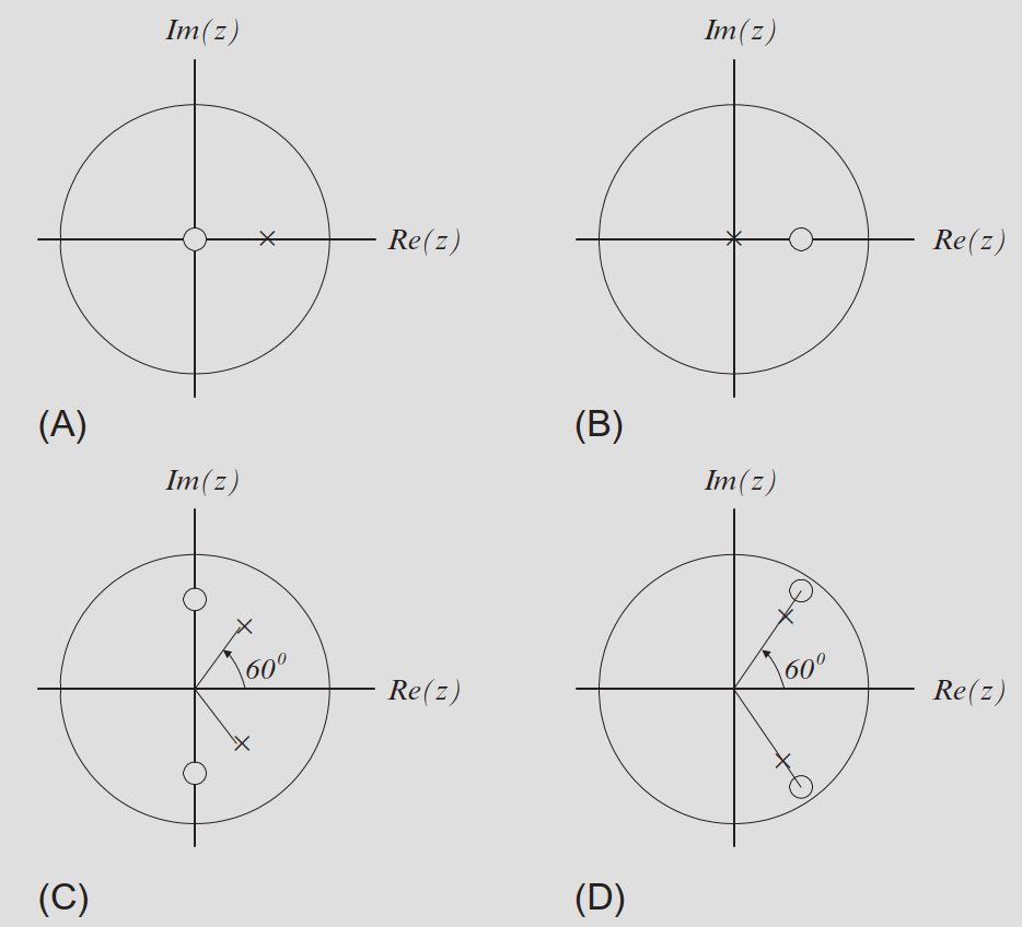
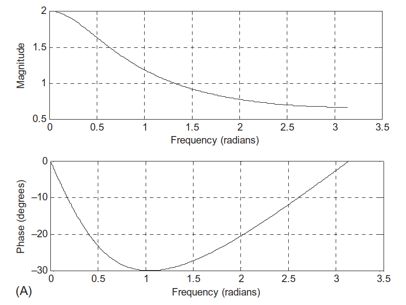
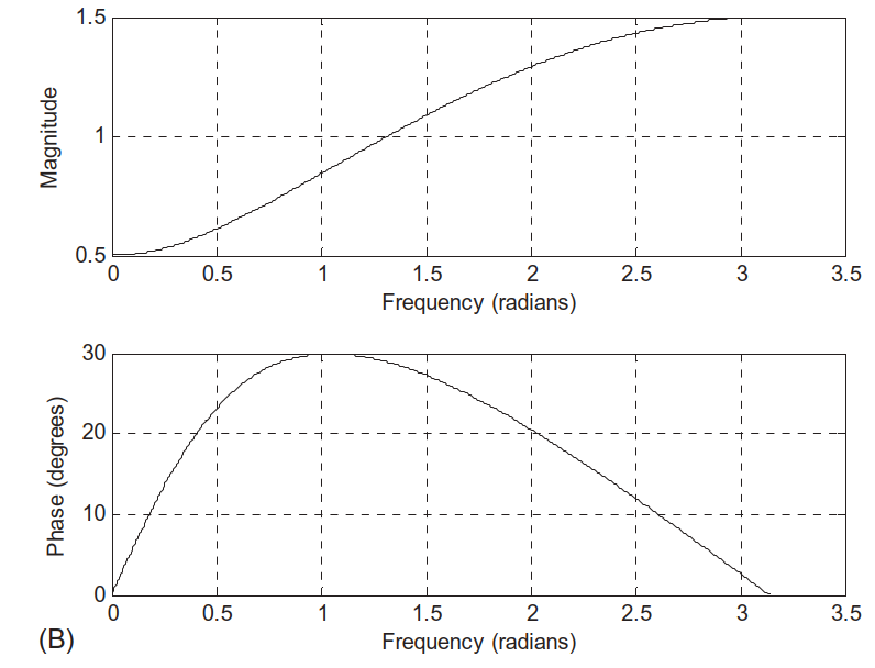
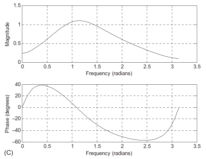
Pole–zero plots are shown in Fig. 6.20:

Fig 6.20: Pole-zero plots of Example 6.12

This is a good time to remind:

• Zeros on or near the unit circle at \(\Omega = 0\) → notch at DC (highpass behavior).
• Zeros at \(\Omega = \pi\) → notch at Nyquist frequency (lowpass behavior).
• Pole–zero patterns in conjugate pairs for real coefficient systems.

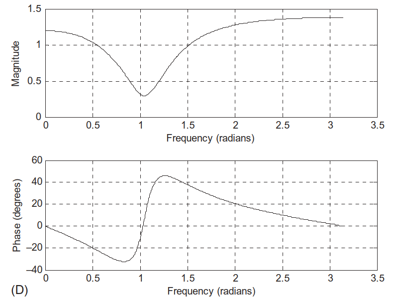
Example 6.12 – MATLAB Code Structure

The textbook Program 6.2 (cleaned up and corrected) looks like:

% Example 6.12

N = 1024;

% Case (a)
B = [1];
A = [1 -0.5];
[h, w] = freqz(B, A, N);
phi = 180*unwrap(angle(h))/pi;
figure(1);
subplot(2,1,1); plot(w, abs(h)); grid;
xlabel('Frequency (rad/sample)'); ylabel('Magnitude');
title('Case (a)');

subplot(2,1,2); plot(w, phi); grid;
xlabel('Frequency (rad/sample)'); ylabel('Phase (degrees)');

% Case (b)
B = [1 -0.5];
A = [1];
[h, w] = freqz(B, A, N);
% ... (similar plotting)

Magnitude + phase plots for each case are shown in Figs. 6.21(a–d).

Fig 6.21 (a)

Fig 6.21 (b)

Fig 6.21 (c)

Fig 6.21 (d)

Mention that the code fragment in the book has variable naming inconsistencies ([hw]=freqz but later uses h, w). Show corrected version and encourage students to always check dimensions and variable names in MATLAB.

Example 6.12 – Identifying Filter Types

From the magnitude responses (Figs. 6.21(a–d)):

• 1. \(H(z) = \dfrac{1}{1 - 0.5 z^{-1}}\)
  • Magnitude is largest at low frequencies, decreases at high frequencies.
  • ⇒ Lowpass filter.
• 2. \(H(z) = 1 - 0.5 z^{-1}\)
  • Zero at \(z = 0.5\) (near DC), magnitude small at low frequencies, larger at high frequencies.
  • ⇒ Highpass filter (simple FIR).

• 3. \(H(z) = \dfrac{0.5 - 0.32 z^{-2}}{1 - 0.5 z^{-1} + 0.25 z^{-2}}\)
  • Band of frequencies where magnitude is significant, low elsewhere.
  • ⇒ Bandpass filter.
• 4. \(H(z) = \dfrac{1 - 0.9 z^{-1} + 0.81 z^{-2}}{1 - 0.6 z^{-1} + 0.36 z^{-2}}\)
  • Narrow band of frequencies attenuated strongly, rest passed.
  • ⇒ Bandstop (bandreject) filter.

Important

Being able to look at a magnitude response and classify the filter type is core. Practice mentally: - Does it pass low, high, a band, or “everything except a band”?

Ask students to think:

• Which of these might be useful for speech preemphasis?
• Which for removing a narrow interference?

Connect (b) to preemphasis (it’s a one‑zero highpass).

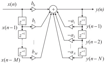
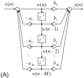
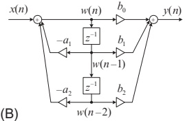
6.6 Realization of Digital Filters – Big Picture

Given a transfer function

\[ H(z) = \frac{B(z)}{A(z)} = \frac{b_0 + b_1 z^{-1} + \dots + b_M z^{-M}}{1 + a_1 z^{-1} + \dots + a_N z^{-N}}, \]

we can implement it in several equivalent ways:

• Direct‑Form I
• Direct‑Form II
• Cascade (Series) of first/second‑order sections
• Parallel sum of first/second‑order sections

All realize the same \(H(z)\) (ideally), but differ in:

• Memory (delay elements) required.
• Numerical behavior (sensitivity to coefficient quantization, overflow).
• Hardware mapping (e.g., how many multipliers/adders).

Emphasize that in real embedded DSP (fixed‑point), the structure matters as much as the polynomial. Many DSP libraries provide second‑order section (SOS) implementations by default.

Direct‑Form I – From Difference Equation

Start from difference equation (time domain):

\[ \begin{aligned} y(n) &= b_0 x(n) + b_1 x(n-1) + \dots + b_M x(n-M) \\ &\quad - a_1 y(n-1) - a_2 y(n-2) - \dots - a_N y(n-N). \end{aligned} \]

Interpretation:

• Feedforward (FIR) part: weighted delayed inputs.
• Feedback (IIR) part: weighted delayed outputs.

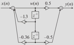
Direct‑Form I structure implements these two parts in parallel, then sums them.

Fig 6.22 (A): Direct-form I realization

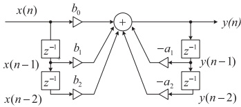
Second‑order example (M = N = 2):

Fig 6.22 (B): Direct-form I with M=2

Fig 6.22 (C): Notation

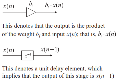
Explain diagram components:

• \(z^{-1}\) = one‑sample delay.
• Multipliers labelled \(b_i\), \(a_j\).
• Adders summing contributions.

Point out that if some \(a_j\) or \(b_i\) are zero, we simply remove those branches.

Direct‑Form II – Reduced Memory

Starting from

\[ Y(z) = H(z) X(z) = \frac{B(z)}{A(z)} X(z), \]

with \(M = N\), rearrange:

\[ Y(z) = B(z) \left( \frac{X(z)}{A(z)} \right). \]

Define an intermediate signal:

\[ W(z) = \frac{X(z)}{1 + a_1 z^{-1} + \dots + a_M z^{-M}}. \]

Then

\[ Y(z) = (b_0 + b_1 z^{-1} + \dots + b_M z^{-M}) W(z). \]

Corresponding difference equations:

• Internal state update: \[ w(n) = x(n) - a_1 w(n-1) - \dots - a_M w(n-M) \]

• Output equation: \[ y(n) = b_0 w(n) + b_1 w(n-1) + \dots + b_M w(n-M) \]

Structure:

Fig 6.23 (A): Direct-form II realization

Second‑order example:

Fig 6.23 (B): Direct-form II with M=2

Note

Direct‑Form II uses fewer delay elements than Direct‑Form I (roughly half when \(M = N\)), which can save memory and hardware.

Explain conceptually: Direct‑Form II “shares” the delay line between feedforward and feedback parts by working on an internal state \(w(n)\) rather than raw \(x(n)\) and \(y(n)\).

Also stress: Direct‑Form II can be more sensitive to coefficient quantization in high‑order filters → reason to use second‑order sections in cascade instead.

Direct‑Form I vs Direct‑Form II – Implementation Trade‑offs

• Number of multiplications: same (same number of \(a_j\) and \(b_i\)).
• Delay elements:
  • Direct‑Form I: two separate delay lines (input and output).
  • Direct‑Form II: one shared delay chain (internal state).
  • ⇒ Direct‑Form II uses fewer delays, saves memory.
• Accumulation & scaling (fixed‑point):
  • Direct‑Form II separates numerator and denominator accumulators.
  • Allows separate scaling to avoid overflow.
• High‑order filters:
  • Better to implement as cascade of second‑order Direct‑Form II sections (biquads).

Ask: In a fixed‑point DSP system, why is overflow dangerous? Answer: Wraparound or saturation can fundamentally distort filter behavior, possibly destabilizing it.

This motivates careful scaling and using second‑order sections rather than monolithic high‑order Direct‑Form II.

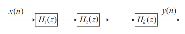
Cascade (Series) Realization – Concept

Factor \(H(z)\) into first‑ and second‑order sections:

\[ H(z) = H_1(z) H_2(z) \cdots H_K(z). \]

Each section \(H_k(z)\) is usually:

• First order: \[ H_k(z) = \frac{b_{k0} + b_{k1} z^{-1}}{1 + a_{k1} z^{-1}} \]

• Or second order: \[ H_k(z) = \frac{b_{k0} + b_{k1} z^{-1} + b_{k2} z^{-2}}{1 + a_{k1} z^{-1} + a_{k2} z^{-2}} \]

Block diagram:

Fig 6.24: Cascade realization

Tip

In practice, high‑order IIR filters are almost always implemented as a cascade of biquads (second‑order sections), each realized by Direct‑Form II (or other numerically robust forms like lattices).

Benefits:

• Better numerical conditioning: errors are “spread out” over sections.
• Poles/zeros can be paired in sections for optimal stability and dynamic range.

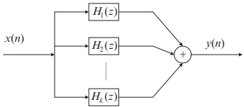
Parallel Realization – Concept

Express \(H(z)\) as a sum of sections:

\[ H(z) = H_1(z) + H_2(z) + \dots + H_K(z). \]

Typically using partial fraction expansion:

• First order: \[ H_k(z) = \frac{b_{k0}}{1 + a_{k1} z^{-1}} \]

• Or second order: \[ H_k(z) = \frac{b_{k0} + b_{k1} z^{-1}}{1 + a_{k1} z^{-1} + a_{k2} z^{-2}} \]

Block diagram:

Fig 6.25: Parallel realization

Parallel form is particularly convenient when:

• Using partial fraction expansion of rational functions.
• Certain sections correspond to specific spectral features you want to modify independently (e.g., adjustable resonances or notches).

However, cascade is more common in standard IIR filter libraries.

Example 6.13 – Given Second‑Order \(H(z)\)

Given:

\[ H(z) = \frac{0.5(1 - z^{-2})}{1 + 1.3 z^{-1} + 0.36 z^{-2}}. \]

Rewrite numerator:

\[ H(z) = \frac{0.5 - 0.5 z^{-2}}{1 + 1.3 z^{-1} + 0.36 z^{-2}}. \]

Identify coefficients:

• \(a_1 = 1.3\), \(a_2 = 0.36\)
• \(b_0 = 0.5\), \(b_1 = 0\), \(b_2 = -0.5\)

We will realize it in:

1. Direct‑Form I and Direct‑Form II.
2. Cascade form via first‑order sections.
3. Parallel form via first‑order sections.

Encourage students to recognize: numerator \(0.5(1 - z^{-2})\) has zeros at \(z = \pm 1\) (DC and Nyquist), i.e., notch at 0 and \(\pi\) rad/sample. Denominator defines a second‑order pole pair.

Example 6.13 – Direct‑Form I

Difference equation (plug coefficients into general form):

\[ \begin{aligned} y(n) &= 0.5 x(n) + 0 \cdot x(n-1) - 0.5 x(n-2) \\ &\quad - 1.3 y(n-1) - 0.36 y(n-2) \\ &= 0.5 x(n) - 0.5 x(n-2) - 1.3 y(n-1) - 0.36 y(n-2). \end{aligned} \]

Direct‑Form I block diagram:

Fig 6.26: Direct-form I realization for Example 6.13

Point out where each coefficient appears in the diagram, and how missing \(x(n-1)\) term simply means that branch is absent.

Ask: For implementation, how many multipliers and delays are needed? (4 multipliers, 4 delays here for M=N=2 in DF‑I).

Example 6.13 – Direct‑Form II

Recall Direct‑Form II equations:

• Internal state: \[ w(n) = x(n) - 1.3 w(n-1) - 0.36 w(n-2) \]

• Output: \[ y(n) = 0.5 w(n) + 0 \cdot w(n-1) - 0.5 w(n-2) = 0.5 w(n) - 0.5 w(n-2). \]

Direct‑Form II structure:

Fig 6.27: Direct-form II realization for Example 6.13

Highlight that now we only have one delay line holding \(w\) states, not separate lines for \(x\) and \(y\). Memory is reduced.

Have students count delays again; note that the number of multipliers is the same as DF‑I.

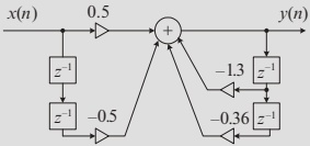
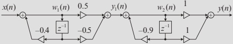
Example 6.13 – Cascade via First‑Order Sections

Factor \(H(z)\) into two first‑order sections:

\[ \begin{aligned} H(z) &= \frac{0.5(1 - z^{-2})}{1 + 1.3 z^{-1} + 0.36 z^{-2}} \\ &= \frac{0.5 - 0.5 z^{-1}}{1 + 0.4 z^{-1}} \cdot \frac{1 + z^{-1}}{1 + 0.9 z^{-1}} \\ &= H_1(z) \cdot H_2(z), \end{aligned} \]

with one possible choice:

• \(H_1(z) = \dfrac{0.5 - 0.5 z^{-1}}{1 + 0.4 z^{-1}}\)
• \(H_2(z) = \dfrac{1 + z^{-1}}{1 + 0.9 z^{-1}}\)

(Other factorizations are possible; this is not unique.)

Cascade structure using Direct‑Form II in each section:

Fig 6.28: Cascade realization for Example 6.13

Explain that we treat each \(H_k(z)\) as a small filter block (biquad or first order), and the full filter is their series connection.

Engineering practice: Implementation libraries (like MATLAB’s sosfilt) take coefficient matrices where each row is one second‑order section.

Example 6.13 – Cascade Difference Equations

Let \(x(n)\) → Section 1 → intermediate \(y_1(n)\) → Section 2 → final \(y(n)\).

Section 1 (\(H_1(z)\)):

\[ \begin{aligned} w_1(n) &= x(n) - 0.4 w_1(n-1) \\ y_1(n) &= 0.5 w_1(n) - 0.5 w_1(n-1) \end{aligned} \]

Section 2 (\(H_2(z)\)):

\[ \begin{aligned} w_2(n) &= y_1(n) - 0.9 w_2(n-1) \\ y(n) &= w_2(n) + w_2(n-1) \end{aligned} \]

Explain variable naming: \(w_1, w_2\) are internal states in each section; \(y_1\) is the internal signal between them.

Ask: Could we swap \(H_1\) and \(H_2\)? Yes; the cascade of LTI systems commutes, though numerical properties may differ in finite precision.

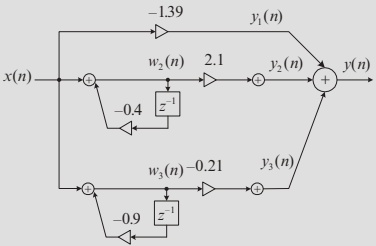
Example 6.13 – Parallel via First‑Order Sections

Use partial fraction expansion. Start by writing:

\[ \frac{H(z)}{z} = \frac{0.5(z^2 - 1)}{z(z + 0.4)(z + 0.9)} = \frac{A}{z} + \frac{B}{z + 0.4} + \frac{C}{z + 0.9}. \]

Solving for \(A, B, C\) (as in the text):

• \(A = -1.39\)
• \(B = 2.1\)
• \(C = -0.21\)

So:

\[ \begin{aligned} H(z) &= -1.39 + \frac{2.1 z}{z + 0.4} - \frac{0.21 z}{z + 0.9} \\ &= -1.39 + \frac{2.1}{1 + 0.4 z^{-1}} + \frac{-0.21}{1 + 0.9 z^{-1}}. \end{aligned} \]

Parallel structure: three sections in parallel, summed at the output.

Fig 6.29: Parallel realization for Example 6.13

Note that the constant term \(-1.39\) can be seen as a “zero order” section: just a gain on \(x(n)\).

Parallel form expresses \(H(z)\) as a sum of simpler modes (like resonances). This can be useful in spectral modeling and for adjustable parametric equalizers.

Example 6.13 – Parallel Difference Equations

Three parallel paths:

1. Constant‑gain path: \[ y_1(n) = -1.39\, x(n) \]

2. First IIR path: \[ \begin{aligned} w_2(n) &= x(n) - 0.4 w_2(n-1) \\ y_2(n) &= 2.1\, w_2(n) \end{aligned} \]

3. Second IIR path: \[ \begin{aligned} w_3(n) &= x(n) - 0.9 w_3(n-1) \\ y_3(n) &= -0.21\, w_3(n) \end{aligned} \]

Total output:

\[ y(n) = y_1(n) + y_2(n) + y_3(n). \]

Highlight: all three branches see the same input \(x(n)\) simultaneously; their outputs are linearly added.

You can see how each term in the partial fraction directly corresponds to a section.

6.7 Applications – Why These Filters Matter

We now apply these concepts to real‑world signals:

1. Preemphasis of speech – simple highpass FIR to boost high frequencies.
2. Bandpass filtering of speech – IIR bandpass filter for a narrow formant region.
3. ECG enhancement with notch filtering – IIR bandstop filter to remove 60 Hz power‑line interference.

Think in terms of:

• What is the signal of interest?
• What is the unwanted component (noise, interference)?
• How do we choose filter type and specs to separate them?

Connect back to the four basic filter types: each of these applications maps naturally to one of them.

Encourage students to think of their project domain (audio, communication, power, biomedical) and picture where filters fit.

6.7.1 Speech Preemphasis – Motivation

Speech spectra typically have more energy at low frequencies and less at high frequencies.

In some applications (e.g., speech coding, recognition):

• Important phonetic information exists at higher frequencies.
• We don’t want encoder/feature extractor to overlook that content.

Solution:

Preemphasis filter – roughly a highpass filter that boosts high frequencies and slightly attenuates low ones.

Simple digital preemphasis filter:

\[ y(n) = x(n) - \alpha x(n-1), \quad 0 < \alpha < 1. \]

Transfer function:

\[ H(z) = 1 - \alpha z^{-1}. \]

• One zero at \(z = \alpha\) (inside unit circle, close to DC).
• Magnitude increases with frequency → highpass behavior.

Emphasize how simple this is: just one subtract and one multiply per sample. Good for hardware or real‑time embedded implementation.

Typically \(\alpha\) between 0.9 and 0.97 in many speech processing systems.

Preemphasis Filter – Frequency Response & Effect

For \(\alpha = 0.9\), \(f_s = 8000\) Hz:

• Use freqz([1 -alpha], 1, 512, fs) to plot frequency response.

Fig 6.30 (A): Frequency responses of preemphasis filter

Effect on speech waveform:

Fig 6.30 (B): Original and preemphasized speech waveforms

Spectra comparison (FFT + Hamming window):

Fig 6.31: Amplitude spectra of original and preemphasized speech

Observation:

• High‑frequency components are boosted.
• Low‑frequency components are relatively attenuated.

Explain that the filter is linear phase (for this single zero it’s not symmetrical FIR, but phase is still well‑behaved for narrowband speech).

Explain briefly the use of windowing (Hamming) in spectrum estimation to reduce leakage.

MATLAB Program 6.3 – Preemphasis Implementation

% Program 6.3: Preemphasis of speech
close all; clear all

fs    = 8000;    % Sampling rate
alpha = 0.9;     % Degree of pre-emphasis

% Frequency response
figure(1);
freqz([1 -alpha], 1, 512, fs);

% Load speech signal
load speech.dat     % Vector 'speech'

% Apply preemphasis filter
y = filter([1 -alpha], 1, speech);

% Time-domain plots
figure(2);
subplot(2,1,1); plot(speech); grid;
ylabel('Speech samples');
title('Original speech');

subplot(2,1,2); plot(y); grid;
ylabel('Filtered samples');
xlabel('Sample index');
title('Preemphasized speech');

% Spectral analysis
figure(3);
N   = length(speech);
Axk = abs(fft(speech .* hamming(N))) / N;
Ayk = abs(fft(y      .* hamming(N))) / N;

f = (0:N/2)*fs/N;
Axk(2:N) = 2*Axk(2:N);
Ayk(2:N) = 2*Ayk(2:N);

subplot(2,1,1); plot(f, Axk(1:N/2+1)); grid;
ylabel('Amplitude spectrum');
title('Original speech');

subplot(2,1,2); plot(f, Ayk(1:N/2+1)); grid;
ylabel('Amplitude spectrum');
xlabel('Frequency (Hz)');
title('Preemphasized speech');

Point out how similar this is to the earlier freqz() example.

Ask students: “If I change alpha to 0.5 or 0.99, how will the spectrum look different?” Encourage them to try this as a quick lab exercise.

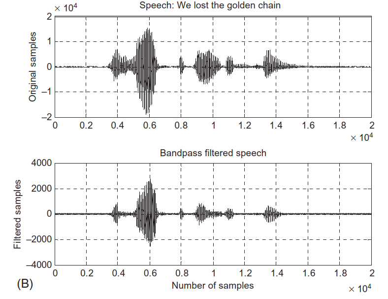
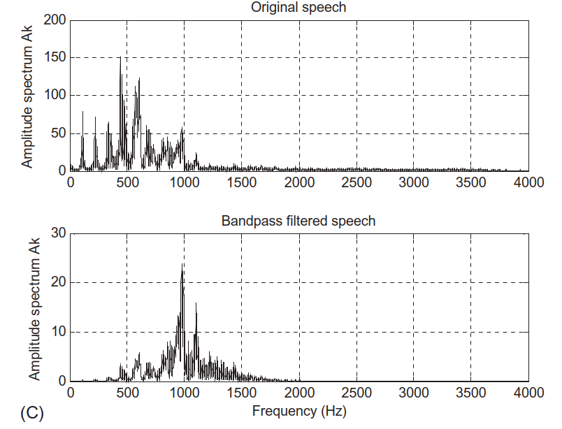
6.7.2 Bandpass Filtering of Speech – Setup

Goal: isolate a narrow band of speech frequencies for analysis or feature extraction.

Given a 4th‑order digital Bandpass Butterworth filter:

• Sampling rate: \(f_s = 8000\) Hz.
• Lower cutoff: 1000 Hz.
• Upper cutoff: 1400 Hz.
• Bandwidth: 400 Hz.

Transfer function:

\[ H(z) = \frac{0.0201 - 0.0402 z^{-2} + 0.0201 z^{-4}}{1 - 2.1192 z^{-1} + 2.6952 z^{-2} - 1.6924 z^{-3} + 0.6414 z^{-4}}. \]

Difference equation:

\[ \begin{aligned} y(n) &= 0.0201 x(n) - 0.0402 x(n-2) + 0.0201 x(n-4) \\ &\quad + 2.1192 y(n-1) - 2.6952 y(n-2) \\ &\quad + 1.6924 y(n-3) - 0.6414 y(n-4). \end{aligned} \]

Highlight that this is a 4th‑order IIR filter; typical to implement as two cascaded biquads in practice (though here given monolithically).

Butterworth ⇒ maximally flat passband (no ripple).

Bandpass Filter – Frequency Response and Effect

Frequency response via freqz:

Fig 6.32 (A): Bandpass filter frequency responses

Time‑domain speech before and after filtering:

Fig 6.32 (B): Original and bandpass filtered speech

Spectra comparison:

Fig 6.32 (C): Spectra of original and bandpass filtered speech

Observation:

• Frequencies below 1000 Hz and above 1400 Hz are significantly attenuated.
• Passband 1000–1400 Hz remains.

Point out that many speech formants (resonant frequencies) lie in certain bands. A bandpass filter can isolate these for pitch or formant analysis.

Ask: “What type of content (e.g., vowel vs consonant) might be emphasized in this band?” This can lead to a discussion of formants.

MATLAB Program 6.4 – Bandpass Filter Implementation

% Program 6.4: Bandpass filtering of speech

fs = 8000;  % Sampling rate

% Bandpass filter coefficients (4th-order)
B = [0.0201 0 -0.0402 0 0.0201];
A = [1 -2.1192 2.6952 -1.6924 0.6414];

% Frequency response
figure(1);
freqz(B, A, 512, fs);
axis([0 fs/2 -40 1]);  % Adjust axis if needed

% Load speech
load speech.dat

% Filter speech
y = filter(B, A, speech);

% Time-domain plots
figure(2);
subplot(2,1,1); plot(speech); grid;
ylabel('Original Samples');
title('Original speech');

subplot(2,1,2); plot(y); grid;
xlabel('Sample index'); ylabel('Filtered Samples');
title('Bandpass filtered speech.');

% Spectral analysis
figure(3);
N   = length(speech);
Axk = abs(fft(speech .* hamming(N)))/N;
Ayk = abs(fft(y      .* hamming(N)))/N;

f = (0:N/2)*fs/N;
Axk(2:N) = 2*Axk(2:N);
Ayk(2:N) = 2*Ayk(2:N);

subplot(2,1,1); plot(f, Axk(1:N/2+1)); grid;
ylabel('Amplitude spectrum');
title('Original speech');

subplot(2,1,2); plot(f, Ayk(1:N/2+1)); grid;
ylabel('Amplitude spectrum');
xlabel('Frequency (Hz)');
title('Bandpass filtered speech');

Encourage students to experiment by changing cutoff frequencies (design new IIR filters using butter or cheby1), and observe how voice quality changes.

This also connects strongly to audio equalization and communication channel filtering.

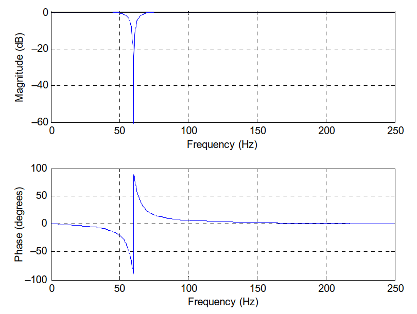
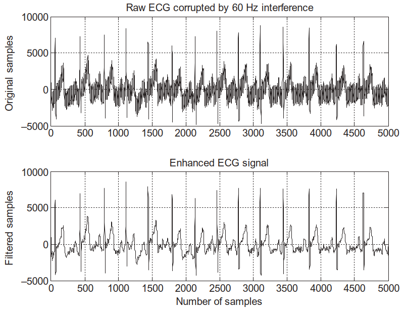
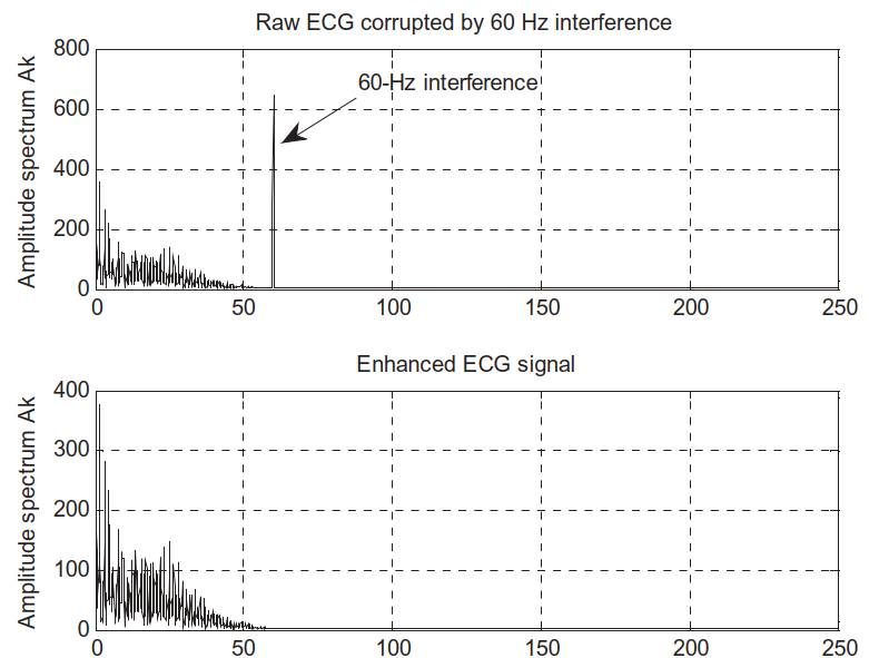
6.7.3 ECG Enhancement with Notch Filter

Problem: ECG signal contaminated by 60 Hz power‑line interference during acquisition.

Given:

• Sampling frequency: \(f_s = 500\) Hz.
• Target: Notch at 60 Hz.

Designed second‑order notch filter:

\[ H(z) = \frac{1 - 1.4579 z^{-1} + z^{-2}}{1 - 1.3850 z^{-1} + 0.9025 z^{-2}}. \]

Difference equation:

\[ y(n) = x(n) - 1.4579 x(n-1) + x(n-2) + 1.3850 y(n-1) - 0.9025 y(n-2). \]

Frequency response:

Fig 6.33: Notch filter frequency responses

Explain that the numerator zeros are placed exactly at the normalized frequency of 60 Hz (and its conjugate), and poles are placed slightly inside the unit circle at almost the same angle, forming a narrow notch.

Normalized notch angle: \(\Omega_0 = 2\pi \cdot 60 / 500\).

ECG Before and After Notch Filtering

Time‑domain ECG:

Fig 6.34: Corrupted and enhanced ECG

• Upper plot: ECG + 60 Hz interference.
• Lower plot: Filtered ECG with notch filter applied.

Frequency‑domain view:

Fig 6.35: Spectra of corrupted and enhanced ECG

• Clear peak at 60 Hz in corrupted signal.
• Peak eliminated in enhanced signal; baseline ECG spectrum preserved.

Important

This is a classic and practical example of DSP in biomedical engineering: a simple, well‑designed digital notch filter significantly improves diagnostic signal quality.

Remind students that in real medical devices, you must preserve morphology of ECG (P‑QRS‑T complex). Too aggressive filtering could distort clinical features.

Thus, filter design balances interference suppression with signal fidelity.

Summary / Key Points

• Four basic digital filter types:
  • Lowpass – passes low frequencies, attenuates high.
  • Highpass – passes high, attenuates low.
  • Bandpass – passes a band, attenuates outside.
  • Bandstop / Notch – attenuates a band, passes outside.
• Filter specs defined by:
  • Passband / stopband edges (\(\Omega_p\), \(\Omega_s\), etc.).
  • Passband ripple \(\delta_p\), stopband ripple \(\delta_s\).
• freqz(B, A, N) computes complex frequency response of \(H(z) = B(z)/A(z)\).

• Realizations of IIR filters:
  • Direct‑Form I – two parallel paths (input and output delays).
  • Direct‑Form II – minimal delays via shared internal state.
  • Cascade – product of first/second‑order sections (common for high orders).
  • Parallel – sum of elementary sections via partial fraction expansion.
• Real ECE applications:
  • Preemphasis of speech – simple highpass FIR filter \(H(z) = 1 - \alpha z^{-1}\).
  • Bandpass speech filter – 4th‑order IIR to isolate 1000–1400 Hz band.
  • ECG enhancement – narrow notch at 60 Hz to remove power‑line interference.

Encourage students to revisit these examples when they see any new filter or DSP device: ask, “What type is it? What realization likely used? What application constraints shaped it?”

These patterns repeat across many ECE sub‑disciplines.

Key Formulas Summary

General IIR transfer function:

\[ H(z) = \frac{B(z)}{A(z)} = \frac{b_0 + b_1 z^{-1} + \dots + b_M z^{-M}}{1 + a_1 z^{-1} + \dots + a_N z^{-N}}. \]

Input–output relation (Direct‑Form I):

\[ \begin{aligned} y(n) &= b_0 x(n) + b_1 x(n-1) + \dots + b_M x(n-M) \\ &\quad - a_1 y(n-1) - \dots - a_N y(n-N). \end{aligned} \]

Direct‑Form II internal state and output:

\[ w(n) = x(n) - a_1 w(n-1) - \dots - a_M w(n-M) \]

\[ y(n) = b_0 w(n) + b_1 w(n-1) + \dots + b_M w(n-M) \]

Preemphasis filter:

\[ y(n) = x(n) - \alpha x(n-1), \quad H(z) = 1 - \alpha z^{-1}. \]

Example bandpass IIR difference equation:

\[ \begin{aligned} y(n) &= 0.0201 x(n) - 0.0402 x(n-2) + 0.0201 x(n-4) \\ &\quad + 2.1192 y(n-1) - 2.6952 y(n-2) \\ &\quad + 1.6924 y(n-3) - 0.6414 y(n-4). \end{aligned} \]

Example ECG notch filter:

\[ H(z) = \frac{1 - 1.4579 z^{-1} + z^{-2}}{1 - 1.3850 z^{-1} + 0.9025 z^{-2}} \]

\[ y(n) = x(n) - 1.4579 x(n-1) + x(n-2) + 1.3850 y(n-1) - 0.9025 y(n-2). \]

Suggest that students create a “formula sheet” including:

• General \(H(z)\) forms.
• Direct‑Form I & II equations.
• Example simple filters (moving average, preemphasis, simple notch).

This will be invaluable in exams and labs.

Quick Interactive Check

1. Suppose you see a magnitude response that is nearly 1 from 0 to \(0.3\pi\), then drops to nearly 0 after \(0.4\pi\). What filter type is this?

2. You are given a speech signal sampled at 8 kHz and want to remove low‑frequency background hum below 200 Hz. What basic filter type would you design?

3. In an ECG system, you see strong narrowband interference at 50 Hz with \(f_s = 500\) Hz. What kind of filter and approximate normalized notch frequency would you choose?

Suggested answers:

1. Lowpass filter.
2. Highpass filter with cutoff around 200 Hz.
3. Notch filter at \(\Omega_0 = 2\pi \cdot 50 / 500 = 0.2\pi\).

Use this slide to gauge understanding and encourage questions.

Interactive Deck

Reminder: freqz vs Direct Computation

In MATLAB we used freqz(B, A, N) to get the frequency response. Here, we’ll do the equivalent in Python using scipy.signal.freqz‑style logic.

We’ll:

1. Define numerator B and denominator A.
2. Evaluate \(H(e^{j\Omega})\) at many points on the unit circle.
3. Plot magnitude and phase.

Interactive: Basic Frequency Response Explorer

Experiment with a simple IIR filter (like Example 6.12).

Try:

• B = [1.0], A = [1.0, -0.5] (Example 6.12(a): lowpass).
• B = [1.0, -0.5], A = [1.0] (Example 6.12(b): highpass).

Reactive: Identify Filter Type from Coefficients

Use sliders to set a simple 2‑tap FIR filter: \(H(z) = b_0 + b_1 z^{-1}\). Observe the magnitude response and guess: lowpass or highpass?

viewof b0 = Inputs.range([-1, 1], {step: 0.1, label: "b0 (feedthrough)"})
viewof b1 = Inputs.range([-1, 1], {step: 0.1, label: "b1 (one-sample delay)"})

Try:

• \(b_0 = 1\), \(b_1 = -0.9\) → highpass / preemphasis‑like.
• \(b_0 = 0.5\), \(b_1 = 0.5\) → lowpass (moving average of length 2).

Interactive: From Difference Equation to Code (Direct‑Form I)

Given the general IIR difference equation:

\[ y(n) = \sum_{k=0}^{M} b_k x(n-k) - \sum_{k=1}^{N} a_k y(n-k). \]

Let’s implement this manually and compare with the vector form.

Try:

• Change x to a step input (x[n] = 1 for all n).
• Observe how the output responds and stabilizes (or not).

Reactive: Direct‑Form II State Evolution

We now implement the Direct‑Form II state update equations with interactive coefficients.

For a second‑order IIR with \(M=2\):

\[ \begin{aligned} w(n) &= x(n) - a_1 w(n-1) - a_2 w(n-2) \\ y(n) &= b_0 w(n) + b_1 w(n-1) + b_2 w(n-2). \end{aligned} \]

viewof a1 = Inputs.range([-2, 2], {step: 0.1, label: "a1 (feedback 1)"})
viewof a2 = Inputs.range([-2, 2], {step: 0.1, label: "a2 (feedback 2)"})
viewof b0_df2 = Inputs.range([-1, 1], {step: 0.1, label: "b0 (feedforward 0)"})
viewof b1_df2 = Inputs.range([-1, 1], {step: 0.1, label: "b1 (feedforward 1)"})
viewof b2_df2 = Inputs.range([-1, 1], {step: 0.1, label: "b2 (feedforward 2)"})

Try to make the filter unstable by choosing \(a_1, a_2\) so that poles move outside the unit circle (e.g., magnitudes > 1). Observe the impulse response growing without bound.

Interactive: Pole–Zero Plot for Example 6.12

Let’s approximate a pole–zero plot for one of the Example 6.12 filters.

Try replacing B and A with other examples ((a), (b), or (d)) and see how poles and zeros move.

Reactive: Preemphasis Filter \(H(z) = 1 - \alpha z^{-1}\)

Recall:

• Preemphasis for speech: \(y(n) = x(n) - \alpha x(n-1)\), \(0 < \alpha < 1\).
• \(H(z) = 1 - \alpha z^{-1}\) is a simple highpass filter.

Use the slider to change \(\alpha\) and observe the magnitude response.

viewof alpha = Inputs.range([0, 0.99], {step: 0.01, label: "Preemphasis α"})

Observe: as \(\alpha\) → 1, the low‑frequency attenuation increases and high‑frequency boost increases.

Interactive: Time‑Domain Preemphasis on Synthetic Signal

Apply preemphasis to a simple synthetic “speech‑like” signal: mixture of low and high frequencies.

Try increasing the amplitude of the high‑frequency component in x and observe how preemphasis modifies the signal.

Reactive: Bandpass Filter – Shape Control

We’ll create a simple FIR bandpass by subtracting a lowpass response from a highpass response. To keep it simple, use two moving-average filters and explore the transition region.

viewof lp_width = Inputs.range([1, 30], {step: 1, label: "Lowpass MA length (L1)"})
viewof hp_width = Inputs.range([1, 30], {step: 1, label: "Highpass MA length (L2)"})

Change L1 and L2 to see how the passband region and transition widths change.

Reactive: Notch Filter at Variable Frequency

Design a simple second‑order notch:

\[ H(z) = \frac{1 - 2r\cos\Omega_0 z^{-1} + r^2 z^{-2}}{1 - 2\cos\Omega_0 z^{-1} + z^{-2}}, \]

where \(\Omega_0\) is the notch frequency and \(0 < r < 1\) controls the width.

viewof f0 = Inputs.range([10, 100], {step: 1, label: "Notch center f0 (Hz)"})
viewof r_notch = Inputs.range([0.5, 0.99], {step: 0.01, label: "Pole radius r"})

Try:

• Set f0 = 60 Hz, r ≈ 0.95 (similar to ECG example).
• Move f0 around and watch the notch move along the frequency axis.

Interactive: Apply Notch Filter to Synthetic ECG + Noise

Create a synthetic ECG‑like waveform (simplified) plus a sinusoidal interference at f0.

Observe how the oscillatory 60 Hz component is suppressed while the slower ECG‑like shape remains.

Try This: Design Your Own Filter

1. Pick a filter type (lowpass, highpass, bandpass, bandstop).
2. Define a simple FIR or low‑order IIR using the code templates above.
3. Plot its magnitude response.
4. Apply it to a synthetic signal (e.g., sum of sinusoids).

Think about:

• Where are the passband and stopband?
• Is the filter stable?
• How many taps or what order does it have?

Use any of the Pyodide cells above as a starting point and modify coefficients, input signals, or sampling rates.