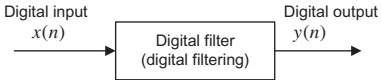
6.1 Basic Filtering Types and Digital Filter Realizations

Digital Signal Processing

Imron Rosyadi

Learning Objectives

By the end of this session, you will be able to:

1. Express a DSP system using a linear constant‑coefficient difference equation.
2. Compute the output of a DSP system recursively (digital filtering) given initial conditions.
3. Derive the transfer function \(H(z)\) from a difference equation (and vice versa).
4. Determine impulse, step, and general system responses using \(H(z)\) and the \(z\)-transform.
5. Plot poles and zeros in the \(z\)-plane and assess BIBO stability.
6. Compute and interpret the digital frequency response \(H(e^{j\Omega})\) (magnitude and phase).

Point out how these objectives map directly to standard DSP design tasks in ECE:

• Implementing an equalizer, noise filter, or control algorithm = specifying a difference equation.
• Verifying stability and response specs = working with poles/zeros and frequency response.

6.1 DSP Systems as Difference Equations

FIG. 6.1 DSP system with input \(x(n)\) and output \(y(n)\).

Key Idea

A (linear, time‑invariant, causal) DSP system (digital filter) with input \(x(n)\) and output \(y(n)\) is described by an \(N\)th‑order linear difference equation:

\[ \begin{aligned} y(n) &= b_{0}x(n) + b_{1}x(n-1) + \cdots + b_{M}x(n-M) \\ &\quad - a_{1}y(n-1) - \cdots - a_{N}y(n-N) \end{aligned} \]

Or compactly:

\[ y(n)=\sum_{i=0}^{M} b_i x(n-i) - \sum_{j=1}^{N} a_j y(n-j) \]

• \(\{b_i\}\): feed‑forward (input) coefficients.
• \(\{a_j\}\): feedback (output) coefficients.
• \(M\), \(N\): input/output orders.

Note

Digital filtering = recursively computing \(y(n)\) from the difference equation, given input \(x(n)\) and initial conditions.

Highlight that this is the discrete‑time analog of an LTI differential equation in analog circuits.

Explain: - “Linear” comes from sums of scaled \(x(\cdot)\) and \(y(\cdot)\). - “Time‑invariant” since the coefficients don’t depend on \(n\). - “Causal” because only present and past samples appear.

Digital filtering is exactly what a microcontroller/DSP chip does for each input sample.

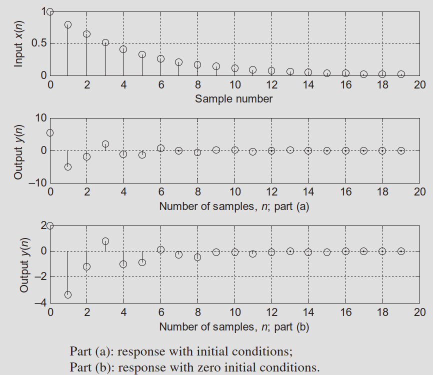
Example 6.1 – Manual Digital Filtering (Nonzero ICs)

System:

\[ y(n) = 0.5\,y(n-2) + x(n-1) \]

Identify coefficients:

• \(N=2\), \(M=1\)
• \(a_1=0,\ a_2=-0.5\)
• \(b_0=0,\ b_1=1\)

Case (a) Nonzero initial conditions:

• \(y(-2)=1,\ y(-1)=0,\ x(-1)=-1\)
• Input \(x(n) = (0.5)^n u(n)\)

Compute for \(n=0,1,2,3\):

\[ \begin{aligned} x(0) &= (0.5)^0 u(0) = 1 \\ y(0) &= 0.5\,y(-2) + x(-1) = 0.5\cdot1 + (-1) = -0.5 \end{aligned} \]

\[ \begin{aligned} x(1) &= 0.5 \\ y(1) &= 0.5\,y(-1) + x(0) = 0.5\cdot0 + 1 = 1.0 \end{aligned} \]

\[ \begin{aligned} x(2) &= 0.25 \\ y(2) &= 0.5\,y(0) + x(1) = 0.5\cdot(-0.5) + 0.5 = 0.25 \end{aligned} \]

\[ \begin{aligned} x(3) &= 0.125 \\ y(3) &= 0.5\,y(1) + x(2) = 0.5\cdot1 + 0.25 = 0.75 \end{aligned} \]

Work through one or two steps on the board, then let students compute the others in pairs.

Key point: initial conditions directly affect early outputs. After some time, the system “forgets” them if it is stable.

Example 6.1 – Effect of Zero Initial Conditions

Case (b) Zero initial conditions:

• \(y(-2)=0,\ y(-1)=0,\ x(-1)=0\)
• Same input: \(x(n) = (0.5)^n u(n)\)

For \(n=0,1,2,3\):

\[ \begin{aligned} x(0) &= 1 \\ y(0) &= 0.5\,y(-2) + x(-1) = 0\cdot1 + 0 = 0 \end{aligned} \]

\[ \begin{aligned} x(1) &= 0.5 \\ y(1) &= 0.5\,y(-1) + x(0) = 0\cdot0 + 1 = 1 \end{aligned} \]

\[ \begin{aligned} x(2) &= 0.25 \\ y(2) &= 0.5\,y(0) + x(1) = 0.5\cdot0 + 0.5 = 0.5 \end{aligned} \]

\[ \begin{aligned} x(3) &= 0.125 \\ y(3) &= 0.5\,y(1) + x(2) = 0.5\cdot1 + 0.25 = 0.75 \end{aligned} \]

Notice:

• Outputs differ at \(n=0,1,2\).
• By \(n=3\), both cases give \(y(3)=0.75\).

Tip

For a stable filter, the effect of initial conditions decays over time.

Connect this to practical ECE applications:

• When turning on a digital audio filter, the first few samples might be “transient” due to initial conditions.
• In simulations, you often ignore an initial transient segment.

Example 6.2 – MATLAB Simulation of a DSP System

System:

\[ y(n) = 2x(n) - 4x(n-1) - 0.5y(n-1) - y(n-2) \]

Initial conditions:

• \(y(-2)=1,\ y(-1)=0,\ x(-1)=-1\)
• Input \(x(n) = (0.8)^n u(n)\)

Goal: compute \(y(n)\) for \(n=0,\dots,19\) using MATLAB.

We pre‑allocate vectors for \(y(n)\) and embed initial conditions as extra entries:

y = zeros(1,20);      % storage for y(0)...y(19)
y = [1 0 y];          % prepend y(-2)=1, y(-1)=0

n = 0:1:19;           % time indices
x = (0.8).^n;         % x(0)...x(19)
x = [0 -1 x];         % prepend x(-2)=0, x(-1)=-1

for n = 1:20
    y(n+2) = 2*x(n+2) - 4*x(n+1) ...
             - 0.5*y(n+1) - 0.5*y(n);
end

Fig. 6.2 Top: input \(x(n)\). Middle: \(y(n)\) with nonzero initial conditions. Bottom: \(y(n)\) with zero initial conditions.

Important teaching points:

• MATLAB indexing with initial conditions: shift by +2 because of \(y(-2)\) and \(y(-1)\).
• Compare plots: the two outputs differ early on but converge later, again illustrating decay of initial conditions in a stable system.

Ask students: based on the plot, does this system seem stable? Why?

Using MATLAB filter() and filtic()

General DSP form:

• Coefficient vectors:

  \[ A = [1\ a_1\ a_2\ \dots\ a_N] \] \[ B = [b_0\ b_1\ b_2\ \dots\ b_M] \]

• Difference equation:

  \[ y(n)=\sum_{i=0}^{M}b_i x(n-i)-\sum_{j=1}^{N} a_j y(n-j) \]

MATLAB syntax with initial conditions:

Zi = filtic(B, A, Yi, Xi);   % compute internal states (direct-form II)
y  = filter(B, A, x, Zi);    % filter operation

• \(X_i = [x(-1)\ x(-2)\ \dots]\)
• \(Y_i = [y(-1)\ y(-2)\ \dots]\)
• \(Z_i = [w(-1)\ w(-2)\ \dots]\): internal delay states

Zero initial conditions:

y = filter(B, A, x);         % Zi defaults to zeros

Note

filtic() maps your physical initial conditions \((x(-k), y(-k))\) into the internal state vector required by the filter() implementation (direct‑form II).

Clarify that the difference equation coefficients \(a_i, b_i\) are what you design, and filter() is just one standard way MATLAB “realizes” the filter.

Mention that direct‑form II realization details will appear later in the chapter, but here we just use the MATLAB black box.

Example 6.1 via MATLAB

Recall system:

• \(y(n) = 0.5\,y(n-2) + x(n-1)\)
• So \(B = [0\ 1]\), \(A = [1\ 0\ -0.5]\).

Case (a) Nonzero initial conditions

• \(x = [1\ 0.5\ 0.25\ 0.125]\) for \(n=0,1,2,3\).
• \(X_i = [x(-1)\ x(-2)\dots] = [-1\ 0]\).
• \(Y_i = [y(-1)\ y(-2)\dots] = [0\ 1]\).

B  = [0 1];
A  = [1 0 -0.5];
x  = [1 0.5 0.25 0.125];
Xi = [-1 0];
Yi = [0 1];

Zi = filtic(B, A, Yi, Xi);
y  = filter(B, A, x, Zi)

Output:

y =
   -0.5000    1.0000    0.2500    0.7500

Case (b) Zero initial conditions

B = [0 1];
A = [1 0 -0.5];
x = [1 0.5 0.25 0.125];

y = filter(B, A, x)

Output:

y =
   0    1.0000    0.5000    0.7500

Emphasize:

• This is exactly how you would simulate your designed filters before coding them into hardware.
• The difference between nonzero and zero initial conditions appears in the first few samples only.

Ask: “Which version corresponds to physically starting the system at rest?” → zero initial conditions.

6.2 From Difference Equation to Transfer Function \(H(z)\)

Given the general LTI difference equation with zero initial conditions:

\[ \begin{aligned} y(n) &= b_0 x(n) + b_1 x(n-1) + \cdots + b_M x(n-M) \\ &\quad - a_1 y(n-1) - \cdots - a_N y(n-N) \end{aligned} \]

Take the \(z\)-transform of both sides, using

• \(Z\{x(n-k)\} = X(z) z^{-k}\)
• \(Z\{y(n-k)\} = Y(z) z^{-k}\)

We obtain:

\[ \begin{aligned} Y(z) &= b_0 X(z) + b_1 X(z) z^{-1} + \cdots + b_M X(z) z^{-M} \\ &\quad - a_1 Y(z) z^{-1} - \cdots - a_N Y(z) z^{-N} \end{aligned} \]

Rearrange:

\[ H(z) = \frac{Y(z)}{X(z)} = \frac{b_0 + b_1 z^{-1} + \cdots + b_M z^{-M}} {1 + a_1 z^{-1} + \cdots + a_N z^{-N}} = \frac{B(z)}{A(z)} \]

with

\[ B(z) = b_0 + b_1 z^{-1} + \cdots + b_M z^{-M} \]

\[ A(z) = 1 + a_1 z^{-1} + \cdots + a_N z^{-N} \]

Important

Transfer function definition

\[ H(z) = \frac{\text{$z$-transform of output}}{\text{$z$-transform of input}} = \frac{Y(z)}{X(z)} \]

This is the central bridge:

• Difference equation ↔︎ transfer function.
• Time domain ↔︎ \(z\)-domain.

Once we have \(H(z)\), we can: - Analyze stability via poles. - Analyze frequency response via \(H(e^{j\Omega})\).

Example 6.3 – Difference Equation → \(H(z)\)

Given:

\[ y(n) = x(n) - x(n-2) - 1.3\,y(n-1) - 0.36\,y(n-2) \]

1. Take \(z\)-transform (zero ICs):

\[ Y(z) = X(z) - X(z)z^{-2} - 1.3 Y(z)z^{-1} - 0.36 Y(z)z^{-2} \]

2. Group \(Y(z)\) and \(X(z)\):

\[ Y(z)\big(1 + 1.3z^{-1} + 0.36z^{-2}\big) = (1 - z^{-2})X(z) \]

3. Transfer function:

\[ H(z) = \frac{Y(z)}{X(z)} = \frac{1 - z^{-2}}{1 + 1.3z^{-1} + 0.36z^{-2}} \]

So:

• \(A(z) = 1 + 1.3z^{-1} + 0.36z^{-2}\)
• \(B(z) = 1 - z^{-2}\)

Point out pattern:

• Terms involving \(y(n-k)\) go to denominator \(A(z)\).
• Terms involving \(x(n-k)\) go to numerator \(B(z)\).

Ask: Is this an IIR or FIR system? → Because of feedback terms \(y(n-1), y(n-2)\), it’s an IIR.

Example 6.4 – FIR System

Given:

\[ y(n) = x(n) - 0.5x(n-1) + 0.36x(n-2) \]

Take \(z\)-transform:

\[ Y(z) = X(z) - 0.5 X(z)z^{-1} + 0.36 X(z)z^{-2} \]

So:

\[ H(z) = \frac{Y(z)}{X(z)} = 1 - 0.5z^{-1} + 0.36z^{-2} \]

• \(A(z) = 1\)
• \(B(z) = 1 - 0.5z^{-1} + 0.36z^{-2}\)

Tip

No feedback terms (\(a_j = 0\)) ⇒ the impulse response has finite length ⇒ FIR filter.

Contrast with Example 6.3.

Mention that FIR filters are always BIBO stable (poles at \(z=0\) only), important in many ECE applications (e.g., precise phase control, linear phase designs).

Example 6.5 – From \(H(z)\) Back to Difference Equation

(a)

Given:

\[ H(z) = \frac{z^{2} - 1}{z^{2} + 1.3z + 0.36} \]

1. Divide numerator/denominator by \(z^2\):

\[ H(z) = \frac{(z^{2}-1)/z^{2}}{(z^{2} + 1.3z + 0.36)/z^{2}} = \frac{1 - z^{-2}}{1 + 1.3z^{-1} + 0.36z^{-2}} \]

2. Write \(Y(z)/X(z)\):

\[ \frac{Y(z)}{X(z)} = \frac{1 - z^{-2}}{1 + 1.3z^{-1} + 0.36z^{-2}} \]

3. Cross‑multiply:

\[ Y(z)(1 + 1.3z^{-1} + 0.36z^{-2}) = X(z)(1 - z^{-2}) \]

4. Inverse \(z\)-transform (using shift property):

\[ y(n) + 1.3 y(n-1) + 0.36 y(n-2) = x(n) - x(n-2) \]

Rearranged:

\[ y(n) = x(n) - x(n-2) - 1.3 y(n-1) - 0.36 y(n-2) \]

Exactly the system from Example 6.3.

(b)

Given:

\[ H(z) = \frac{z^{2} - 0.5z + 0.36}{z^{2}} \]

Divide by \(z^{2}\):

\[ H(z) = \frac{Y(z)}{X(z)} = 1 - 0.5z^{-1} + 0.36z^{-2} \]

Thus:

\[ Y(z) = X(z) - 0.5 z^{-1}X(z) + 0.36 z^{-2}X(z) \]

Inverse \(z\)-transform:

\[ y(n) = x(n) - 0.5 x(n-1) + 0.36 x(n-2) \]

Same as Example 6.4.

This pair of examples reinforces the two‑way mapping between time and \(z\)-domain descriptions.

Practical note: in filter design tools (MATLAB, Python), you often specify \(H(z)\) (coeff vectors A,B) and then the implementation executes the equivalent difference equation sample by sample.

Factorized Pole–Zero Form of \(H(z)\)

Any rational \(H(z)\) can be factored as:

\[ H(z) = \frac{b_0 (z - z_1)(z - z_2)\cdots(z - z_M)} {(z - p_1)(z - p_2)\cdots(z - p_N)} \]

• \(\{z_i\}\): zeros (roots of numerator).
• \(\{p_i\}\): poles (roots of denominator).

Example 6.6

Given:

\[ H(z) = \frac{1 - z^{-2}}{1 + 1.3z^{-1} + 0.36 z^{-2}} \]

Multiply numerator & denominator by \(z^{2}\):

\[ H(z) = \frac{z^{2} - 1}{z^{2} + 1.3z + 0.36} \]

Solve roots:

• \(z^{2} - 1 = 0 \Rightarrow z = 1,\ -1\) (zeros).
• \(z^{2} + 1.3z + 0.36 = 0 \Rightarrow z = -0.4,\ -0.9\) (poles).

Pole–zero form:

\[ H(z) = \frac{(z - 1)(z + 1)}{(z + 0.4)(z + 0.9)} \]

Explain that plotting these poles and zeros in the \(z\)-plane gives powerful geometric intuition about stability and frequency response.

Zeros “push down” magnitude near their angles; poles “pull up” magnitude.

6.2.1 Impulse, Step, and System Responses

Impulse response \(h(n)\)

• Response to input \(x(n) = \delta(n)\).

• With \(X(z) = Z\{\delta(n)\} = 1\):

  \[ h(n) = Z^{-1}\{H(z) X(z)\} = Z^{-1}\{H(z)\} \]

Step response (to \(x(n)=u(n)\), zero ICs):

• \(X(z) = Z\{u(n)\} = \dfrac{z}{z-1}\).

  \[ y(n) = Z^{-1}\Big\{ H(z) \frac{z}{z-1} \Big\} \]

General system response to arbitrary \(x(n)\):

• In \(z\)-domain:

  \[ Y(z) = H(z) X(z) \]

• In time domain:

  \[ y(n) = Z^{-1}\{Y(z)\} \]

Note

Equivalently, in time domain, for LTI systems:

\[ y(n) = (h * x)(n) = \sum_{k=-\infty}^{\infty} h(k)\,x(n-k) \]

(convolution).

Relate this to circuit theory:

• Impulse response ↔︎ unit impulse response of an LTI system.
• Step response ↔︎ standard test used for characterizing systems (e.g., step response of amplifiers or control systems).

Here we exploit the convenience of \(z\)-transform algebra instead of doing convolution by hand.

Example 6.7 – Responses of a First‑Order System

System transfer function:

\[ H(z) = \frac{z+1}{z-0.5} \]

We will find:

1. Impulse response \(h(n)\).
2. Step response to \(x(n)=u(n)\).
3. Response to \(x(n) = (0.25)^n u(n)\).

6.7 (a) Impulse Response

We rewrite:

\[ \frac{H(z)}{z} = \frac{z+1}{z(z-0.5)} = \frac{A}{z} + \frac{B}{z-0.5} \]

Find residues:

• At \(z=0\):

  \[ A = \left. \frac{z+1}{z-0.5} \right|_{z=0} = \frac{0+1}{0-0.5} = -2 \]

• At \(z=0.5\):

  \[ B = \left. \frac{z+1}{z} \right|_{z=0.5} = \frac{1.5}{0.5} = 3 \]

Thus:

\[ \frac{H(z)}{z} = -\frac{2}{z} + \frac{3}{z-0.5} \]

Multiply both sides by \(z\):

\[ H(z) = -2 + \frac{3z}{z-0.5} \]

Inverse \(z\)-transform:

• \(-2 \leftrightarrow -2\,\delta(n)\).
• \(\dfrac{z}{z-0.5} \leftrightarrow (0.5)^n u(n)\).

So:

\[ h(n) = -2\,\delta(n) + 3 (0.5)^n u(n) \]

6.7 (b) Step Response

Step input: \(x(n) = u(n)\), \(X(z) = \dfrac{z}{z-1}\).

Thus:

\[ Y(z) = H(z) X(z) = \frac{z+1}{z-0.5}\cdot\frac{z}{z-1} \]

Write:

\[ \frac{Y(z)}{z} = \frac{z+1}{(z-0.5)(z-1)} = \frac{A}{z-0.5} + \frac{B}{z-1} \]

Residues:

• At \(z=0.5\):

  \[ A = \left. \frac{z+1}{z-1} \right|_{z=0.5} = \frac{1.5}{-0.5} = -3 \]

• At \(z=1\):

  \[ B = \left. \frac{z+1}{z-0.5} \right|_{z=1} = \frac{2}{0.5} = 4 \]

So:

\[ Y(z) = \frac{-3z}{z-0.5} + \frac{4z}{z-1} \]

Inverse \(z\)-transform:

• \(\dfrac{z}{z-0.5} \leftrightarrow (0.5)^n u(n)\).
• \(\dfrac{z}{z-1} \leftrightarrow u(n)\).

Hence step response:

\[ y(n) = -3 (0.5)^n u(n) + 4 u(n) \]

6.7 (c) Response to \(x(n) = (0.25)^n u(n)\)

Input:

\[ X(z) = Z\{(0.25)^n u(n)\} = \frac{z}{z-0.25} \]

Then:

\[ Y(z) = H(z) X(z) = \frac{z+1}{z-0.5}\cdot\frac{z}{z-0.25} = \frac{z(z+1)}{(z-0.5)(z-0.25)} \]

Partial fraction:

\[ \frac{Y(z)}{z} = \frac{z+1}{(z-0.5)(z-0.25)} = \frac{A}{z-0.5} + \frac{B}{z-0.25} \]

Solving yields:

\[ Y(z) = \frac{6z}{z-0.5} - \frac{5z}{z-0.25} \]

Inverse \(z\)-transform:

\[ y(n) = 6(0.5)^n u(n) - 5(0.25)^n u(n) \]

Fig. 6.4 Impulse, step, and system response in Example 6.7.

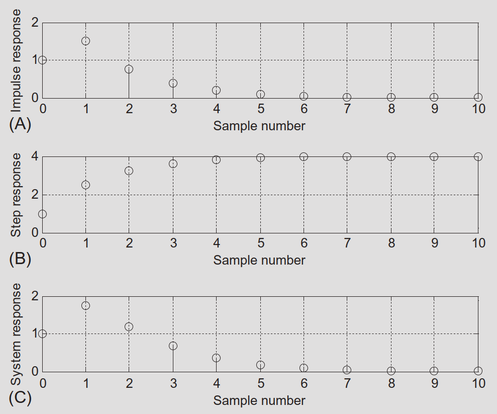
• Top: impulse response \(h(n)\).
• Middle: step response.
• Bottom: response to \((0.25)^n u(n)\).

Use this example to reinforce:

• Partial fractions in the \(z\)-domain lead directly to standard sequences.
• Poles at \(0.5\) and \(0.25\) cause exponential decays in time.

Ask: Is the system stable? (Yes, |0.5|<1).

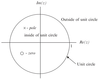
6.3 The \(z\)-Plane Pole–Zero Plot and Stability

z-plane basics

• Horizontal axis: \(\Re\{z\}\).
• Vertical axis: \(\Im\{z\}\).
• The unit circle \(|z|=1\) divides the plane.
• Poles: marked with “×”.
• Zeros: marked with “○”.

We plot poles and zeros of \(H(z)\) to analyze:

• Stability (pole locations).
• Frequency response shape.

Fig. 6.5 Example z-plane with poles and zeros.

Emphasize that many DSP design tools visualise pole–zero plots because they give immediate insight:

• Poles near the unit circle → sharp resonances.
• Zeros on the unit circle → sharp notches.

Especially important in control, audio equalization, and communication filters.

Example 6.8 – Pole–Zero Plot

Given:

\[ H(z) = \frac{z^{-1}-0.5z^{-2}}{1 + 1.2z^{-1} + 0.45z^{-2}} \]

Convert to advanced form (positive powers) by multiplying numerator and denominator by \(z^{2}\):

\[ H(z) = \frac{(z^{-1}-0.5z^{-2})z^{2}}{(1+1.2z^{-1}+0.45z^{-2})z^{2}} = \frac{z - 0.5}{z^{2} + 1.2z + 0.45} \]

Find zeros and poles:

• Zero: solve \(z - 0.5 = 0\) ⇒ \(z_1 = 0.5\).

• Poles: solve \(z^{2} + 1.2z + 0.45 = 0\):

  \[ p_1 = -0.6 + j0.3,\quad p_2 = -0.6 - j0.3 \]

Magnitude of poles:

\[ |p_{1,2}| = \sqrt{(-0.6)^2 + (0.3)^2} \approx 0.671 < 1 \]

So poles are inside the unit circle.

Fig. 6.6 The z-plane pole-zero plot of Example 6.8.

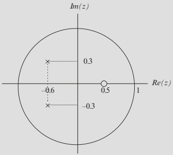
Pole–zero form:

\[ H(z) = \frac{z-0.5}{(z + 0.6 - j0.3)(z + 0.6 + j0.3)} \]

Ask students to comment:

• Are the poles stable? (Yes, inside unit circle).
• How do the complex conjugate poles suggest oscillatory decaying behavior in the impulse response?

Connect to second‑order resonant behavior in analog circuits (underdamped response).

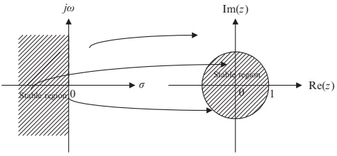
Mapping Between \(s\)-Plane and \(z\)-Plane

Continuous‑time sampled signal (sampling period \(T\)):

\[ x_s(t) = \sum_{n=0}^{\infty} x(nT)\,\delta(t-nT) \]

Laplace transform: using \(L\{\delta(t-nT)\}=e^{-nTs}\):

\[ X_s(s) = \sum_{n=0}^{\infty} x(nT)e^{-nTs} \]

One‑sided \(z\)-transform of sequence \(x(n)\):

\[ X(z) = \sum_{n=0}^{\infty} x(n) z^{-n} \]

Comparing terms, we see the mapping:

\[ z = e^{sT} \]

Let \(s = -\alpha \pm j\omega\):

\[ z = e^{-\alpha T \pm j\omega T} = e^{-\alpha T} \angle \pm\omega T \]

Conclusions:

• \(\alpha > 0\) ⇒ left half \(s\)-plane (stable continuous system) maps to \(|z| = e^{-\alpha T} < 1\) = inside the unit circle.
• \(\alpha = 0\) ⇒ \(s = j\omega\) axis maps to \(|z|=1\) = unit circle.
• \(\alpha < 0\) ⇒ unstable continuous poles map outside unit circle.

FIG. 6.8 Mapping between s-plane and z-plane.

Stress the powerful analogy:

• Stable analog LTI systems have poles in LHHP.
• Stable digital LTI systems have poles inside the unit circle.

This is heavily used in transforming analog filter designs into digital ones (bilinear transform, impulse invariance, etc.).

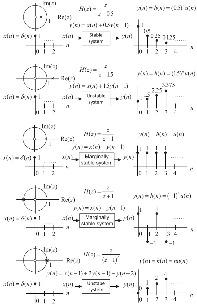
Stability Rules for DSP Systems

A digital system is BIBO stable if every bounded input produces a bounded output.

For a rational \(H(z)\), stability is determined by pole locations:

1. Stable:
   • All poles of \(H(z)\) are inside the unit circle.
2. Unstable:
   • At least one pole is outside the unit circle.
3. Marginally stable:
   • Outermost pole(s) lie on the unit circle and are first‑order.
4. Unstable (special case):
   • Outermost pole(s) on the unit circle are multiple‑order (e.g., double pole).
5. Zeros do not affect stability (only poles matter).

Illustrations in Fig. 6.9:

Fig. 6.9 Stability illustrations.

Tie back to impulse response:

• Stable: \(h(n)\) decays to zero.
• Unstable: \(h(n)\) grows without bound.
• Marginally stable: \(h(n)\) oscillates but does not decay (constant amplitude sinusoid).

Ask: Why do multiple poles on the unit circle produce unbounded growth? → polynomial growth multiplied by sinusoid.

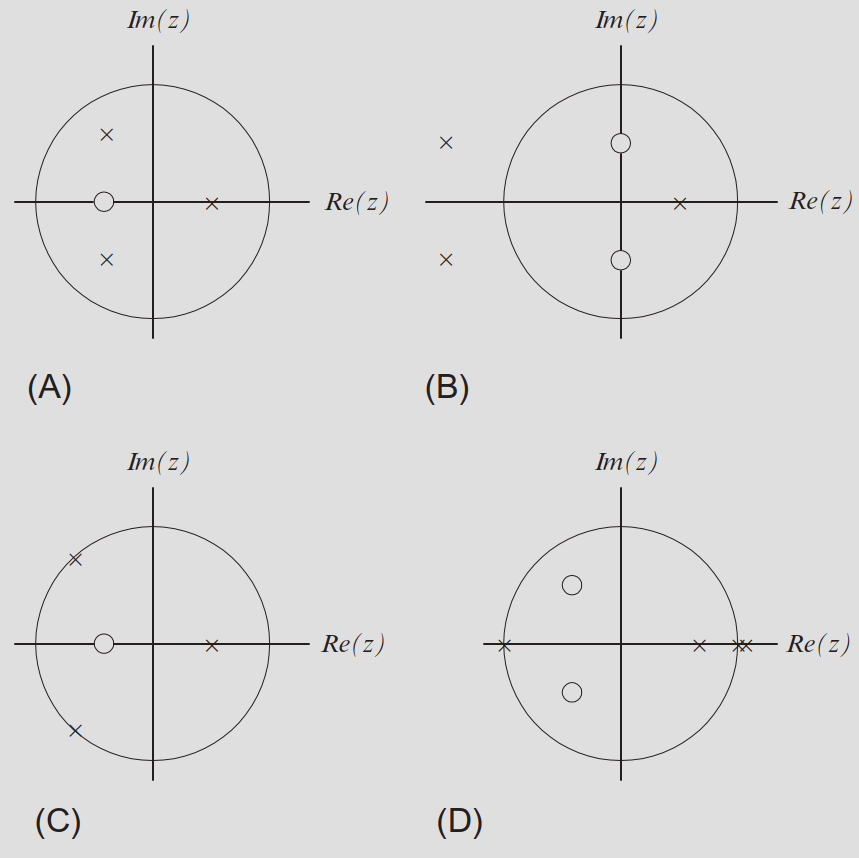
Example 6.9 – Stability from Pole–Zero Plots

We are given several transfer functions and asked to:

• Sketch z‑plane pole–zero plots.
• Determine stability.

(a)

\[ H(z) = \frac{z+0.5}{(z-0.5)(z^2 + z + 0.5)} \]

• Zero: \(z=-0.5\).
• Poles:

  • \(z=0.5\), \(|z|=0.5 < 1\).

  • Roots of \(z^2 + z + 0.5 = 0\):

    \[ z = -0.5 \pm j0.5,\quad |z| = \sqrt{0.5^2 + 0.5^2} \approx 0.707 < 1 \]

All poles inside unit circle ⇒ stable.

(b)

\[ H(z) = \frac{z^2 + 0.25}{(z-0.5)(z^2 + 3z + 2.5)} \]

• Zeros: \(z = \pm j0.5\).
• Poles:

  • \(z=0.5\), \(|z|=0.5<1\).

  • Roots of \(z^2 + 3z + 2.5 = 0\):

    \[ z = -1.5 \pm j0.5,\quad |z| \approx 1.581 > 1 \]

Some poles outside unit circle ⇒ unstable.

(c)

\[ H(z) = \frac{z+0.5}{(z-0.5)(z^2 + 1.4141z + 1)} \]

• Zero: \(z=-0.5\).
• Poles:

  • \(z = 0.5,\ |z|=0.5<1\).

  • Roots of \(z^2 + 1.4141z + 1 = 0\):

    \[ z \approx -0.707 \pm j0.707,\quad |z|\approx 1 \]

Outermost poles on unit circle, first order ⇒ marginally stable.

(d)

\[ H(z) = \frac{z^{2}+z+0.5}{(z-1)^2 (z+1)(z-0.6)} \]

• Zeros: \(z = -0.5 \pm j0.5\).
• Poles:
  • \(z=1\) (double pole), \(|z|=1\).
  • \(z=-1\), \(|z|=1\).
  • \(z=0.6\), \(|z|=0.6<1\).

Outermost pole at \(z=1\) is second order on unit circle ⇒ unstable.

Fig. 6.10 Pole-zero plots for Example 6.9.

Use this to reinforce:

• Zeros can be anywhere; they don’t affect stability.
• Multiple poles on the unit circle are dangerous (unbounded response).

Relate to oscillators: e.g., a perfect oscillator corresponds to a pole on the unit circle; in practice, any slight pole radius > 1 yields growing amplitude.

6.4 Digital Filter Frequency Response

From analog to digital frequency response:

• Analog LTI system: \(H(s)\).
• Steady‑state frequency response: \(H(j\omega) = H(s)\big|_{s=j\omega}\).

For digital systems:

• Use mapping \(z = e^{sT}\).
• On \(j\omega\) axis → \(z = e^{j\omega T}\).

Thus digital frequency response:

\[ H(e^{j\omega T}) = H(z)\big|_{z=e^{j\omega T}} = \big|H(e^{j\omega T})\big| \angle H(e^{j\omega T}) \]

Define normalized digital radian frequency:

\[ \Omega = \omega T \]

Then we write:

\[ H(e^{j\Omega}) = H(z)\big|_{z=e^{j\Omega}} = \big|H(e^{j\Omega})\big| \angle H(e^{j\Omega}) \]

Note

In DSP, we typically work with \(\Omega \in [0,\pi]\) radians, corresponding to physical frequencies \(f \in [0, f_s/2]\).

Emphasize that \(H(e^{j\Omega})\) is obtained by evaluating the transfer function on the unit circle in the \(z\)-plane.

This is the key link between pole–zero plots and frequency response.

Transient vs Steady‑State Response to a Sinusoid

Consider a digital filter with transfer function \(H(z)\) and sinusoidal input:

• Input amplitude: \(K\).
• Frequency: \(\Omega\).

Fig. 6.11 System transient and steady-state frequency responses.

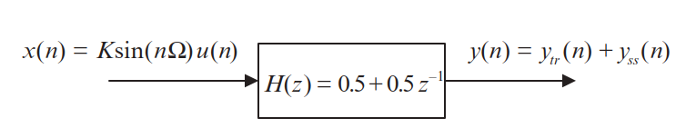
We can show (by partial fractions and inverse \(z\)-transform, as in the text) that the output has form:

\[ y(n) = y_{tr}(n) + y_{ss}(n) \]

where

• \(y_{tr}(n)\): transient response (decays with \(n\) for a stable system).
• \(y_{ss}(n)\): steady‑state sinusoid at same frequency.

General steady‑state result:

For input \(x(n) = K\sin(\Omega n)\,u(n)\),

\[ y_{ss}(n) = K\big|H(e^{j\Omega})\big| \sin\big(n\Omega + \angle H(e^{j\Omega})\big)u(n) \]

So:

• Magnitude response: \(|H(e^{j\Omega})|\) = ratio of output amplitude to input amplitude.
• Phase response: \(\angle H(e^{j\Omega})\) = phase shift between output and input.

Fig. 6.12 Digital filter responses to different input sinusoids.

This is the discrete‑time analog of sinusoidal steady state in AC circuit analysis.

Once the transient dies out, the filter simply scales and phase‑shifts the sinusoid at each frequency.

Use this to motivate why we care so much about \(|H(e^{j\Omega})|\) and \(\angle H(e^{j\Omega})\).

Properties of \(H(e^{j\Omega})\)

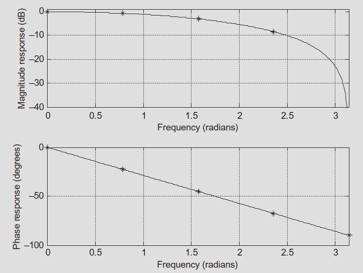
1. Periodicity

From Euler’s identity:

\[ e^{j(\Omega + k2\pi)} = e^{j\Omega} \]

for integer \(k\). Thus:

• \(H(e^{j\Omega}) = H(e^{j(\Omega + k2\pi)})\).
• \(|H(e^{j\Omega})| = |H(e^{j(\Omega + k2\pi)})|\).
• \(\angle H(e^{j\Omega}) = \angle H(e^{j(\Omega + k2\pi)})\).

2. Symmetry (for real‑coefficient filters)

• Magnitude: \(|H(e^{-j\Omega})| = |H(e^{j\Omega})|\).
• Phase: \(\angle H(e^{-j\Omega}) = -\angle H(e^{j\Omega})\).

Because of sampling:

• Maximum useful frequency is the folding frequency \(f_s/2\).

• Corresponding normalized radian frequency:

  \[ \Omega = \omega T = 2\pi \frac{f_s}{2} T = \pi \]

Thus we only need \(\Omega \in [0,\pi]\).

Conversion to Hz:

\[ f = \frac{\Omega}{2\pi} f_s \]

Magnitude in decibels:

\[ |H(e^{j\Omega})|_{\text{dB}} = 20\log_{10}\big(|H(e^{j\Omega})|\big) \]

Explain that in most practical plots (MATLAB freqz), you see \(0\) to \(\pi\) on the horizontal axis.

Relate decibels to power/range constraints in communication, audio, and RF design.

Example 6.10 – Frequency Response of a Simple Averager (Lowpass)

System:

\[ y(n) = 0.5x(n) + 0.5x(n-1) \]

This is a 2‑point moving average with equal weights.

1. \(z\)-transform:

\[ Y(z) = 0.5X(z) + 0.5z^{-1}X(z) \]

2. Transfer function:

\[ H(z) = \frac{Y(z)}{X(z)} = 0.5 + 0.5z^{-1} \]

3. Frequency response: substitute \(z=e^{j\Omega}\):

\[ \begin{aligned} H(e^{j\Omega}) &= 0.5 + 0.5 e^{-j\Omega} \\ &= 0.5 + 0.5\cos\Omega - j0.5\sin\Omega \end{aligned} \]

4. Magnitude and phase:

\[ |H(e^{j\Omega})| = \sqrt{(0.5+0.5\cos\Omega)^2 + (0.5\sin\Omega)^2} \]

\[ \angle H(e^{j\Omega}) = \tan^{-1}\left(\frac{-0.5\sin\Omega}{0.5+0.5\cos\Omega}\right) \]

Example 6.10 – Numerical Values

Sampling rate \(f_s = 8000\) Hz.

\(\Omega\) (rad)	\(f = \frac{\Omega}{2\pi}f_s\) (Hz)	\(|H(e^{j\Omega})|\)	\(|H(e^{j\Omega})|_{\text{dB}}\)	\(\angle H(e^{j\Omega})\)
0	0	1.000	0 dB	\(0^\circ\)
\(0.25\pi\)	1000	0.924	−0.687 dB	−22.5°
\(0.50\pi\)	2000	0.707	−3.012 dB	−45°
\(0.75\pi\)	3000	0.383	−8.336 dB	−67.5°
\(1.00\pi\)	4000	0.000	−∞	−90°

Fig. 6.13 Frequency responses of the digital filter in Example 6.10.

• As frequency increases, magnitude decreases.
• Filter passes low frequencies, attenuates high frequencies ⇒ lowpass filter.
• Phase is approximately linear in the main band.

Ask students:

• What does this do to a noisy ECG signal? (Averaging smooths out high‑frequency noise.)
• Why does \(|H(e^{j\pi})|=0\)? (At Nyquist, consecutive samples differ by a sign; averaging cancels.)

Example 6.10 – Periodicity and Symmetry

Using \(\Omega = 0.25\pi + 2\pi\):

\[ |H(e^{j(0.25\pi + 2\pi)})| = |H(e^{j0.25\pi})| = 0.924 \]

\[ \angle H(e^{j(0.25\pi + 2\pi)}) = \angle H(e^{j0.25\pi}) = -22.5^\circ \]

Using \(\Omega = -0.25\pi\):

\[ |H(e^{-j0.25\pi})| = |H(e^{j0.25\pi})| = 0.924 \]

\[ \angle H(e^{-j0.25\pi}) = -\angle H(e^{j0.25\pi}) = +22.5^\circ \]

Fig. 6.14 Periodicity of the magnitude response and phase response in Example 6.10.

• Magnitude and phase are periodic with \(2\pi\).
• Over \([- \pi, \pi]\): magnitude is even, phase is odd.

Note the “sawtooth” phase plot due to phase wrapping. The underlying phase is linear in \(\Omega\), but when it exceeds \(\pi\) or \(-\pi\), plotting software wraps it back.

This is important in practice when interpreting phase plots from tools like MATLAB freqz.

Example 6.11 – First‑Order Highpass‑Like Response

System:

\[ y(n) = x(n) - 0.5 y(n-1) \]

1. \(z\)-transform:

\[ Y(z) = X(z) - 0.5z^{-1}Y(z) \]

2. Transfer function:

\[ H(z) = \frac{Y(z)}{X(z)} = \frac{1}{1 + 0.5z^{-1}} = \frac{z}{z + 0.5} \]

3. Frequency response: \(z = e^{j\Omega}\):

\[ H(e^{j\Omega}) = \frac{1}{1 + 0.5e^{-j\Omega}} = \frac{1}{1 + 0.5\cos\Omega - j0.5\sin\Omega} \]

4. Magnitude and phase:

\[ |H(e^{j\Omega})| = \frac{1}{\sqrt{(1+0.5\cos\Omega)^2 + (0.5\sin\Omega)^2}} \]

\[ \angle H(e^{j\Omega}) = -\tan^{-1}\left(\frac{-0.5\sin\Omega}{1+0.5\cos\Omega}\right) \]

Example 6.11 – Numerical Values

Sampling rate \(f_s = 8000\) Hz.

\(\Omega\) (rad)	\(f=\frac{\Omega}{2\pi}f_s\) (Hz)	\(|H(e^{j\Omega})|\)	\(|H(e^{j\Omega})|_{\text{dB}}\)	\(\angle H(e^{j\Omega})\)
0	0	0.670	−3.479 dB	\(0^\circ\)
\(0.25\pi\)	1000	0.715	−2.914 dB	14.64°
\(0.50\pi\)	2000	0.894	−0.973 dB	26.57°
\(0.75\pi\)	3000	1.357	2.652 dB	28.68°
\(1.00\pi\)	4000	2.000	6.021 dB	\(0^\circ\)

Fig. 6.15 Frequency responses of the digital filter in Example 6.11.

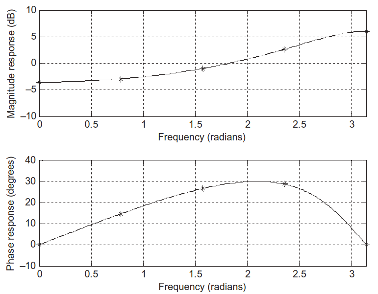
• Magnitude increases with frequency ⇒ highpass‑like behavior.
• Useful for removing low‑frequency drift (e.g., sensor bias).

Compare this system’s behavior to an analog highpass RC filter used to remove DC components.

Ask: what happens to constant input \(x(n)=C\)? → It decays over time due to feedback term.

FIR vs IIR Systems

Starting from the general difference equation:

\[ y(n) = \sum_{i=0}^{M} b_i x(n-i) - \sum_{j=1}^{N} a_j y(n-j) \]

• If all \(a_j = 0\), we get:

  \[ y(n) = \sum_{i=0}^{M} b_i x(n-i) \]

  • The impulse response \(h(n)\) is just \(\{b_0, b_1, \dots, b_M\}\), and zero outside that range.
  • Finite‑length \(h(n)\) ⇒ Finite Impulse Response (FIR).
  • \(H(z) = B(z)\) with denominator \(A(z) = 1\).

• If any \(a_j \neq 0\):

  • Impulse response \(h(n)\) generally has infinite duration.
  • \(H(z) = \dfrac{B(z)}{A(z)}\), \(A(z) \neq 1\).
  • This is an Infinite Impulse Response (IIR) filter.

Tip

Summary

• FIR: no feedback, always BIBO stable, often used for linear‑phase designs.
• IIR: uses feedback, can achieve sharp responses with fewer coefficients, but stability must be checked (poles inside unit circle).

Connect to real‑world ECE choices:

• Audio EQ on phones often uses IIR (biquad sections) for efficiency.
• High‑precision measurement filters or multirate filters often use FIR to guarantee linear phase and stability.

Summary / Key Points

1. Difference equations are the time‑domain description of DSP systems (digital filters), involving past and present inputs and outputs.
2. Digital filtering = recursively computing \(y(n)\) from the difference equation and initial conditions.
3. The transfer function \(H(z) = \dfrac{Y(z)}{X(z)} = \dfrac{B(z)}{A(z)}\) fully characterizes an LTI discrete‑time system in the \(z\)-domain.
4. You can convert between difference equations and \(H(z)\) (via \(z\)-transform and its inverse).
5. Impulse response \(h(n)\) is \(Z^{-1}\{H(z)\}\).
   • Step and general responses follow from \(Y(z) = H(z)X(z)\) and inverse \(z\)-transform.

6. Poles and zeros plotted in the \(z\)-plane determine stability and shape the frequency response.
   • Stable: all poles inside unit circle.
   • Marginally stable: outer poles on unit circle, first order.
   • Unstable: any pole outside unit circle or multiple poles on unit circle.
7. The digital frequency response is \(H(e^{j\Omega}) = H(z)\big|_{z=e^{j\Omega}}\):
   • \(|H(e^{j\Omega})|\) gives gain vs frequency.
   • \(\angle H(e^{j\Omega})\) gives phase shift vs frequency.
8. FIR filters (no feedback) have finite impulse responses and are always stable; IIR filters (with feedback) have infinite impulse responses and require pole‑location stability checks.

Re‑emphasize practical implications:

• When designing a filter, we’ll specify desired amplitude/phase responses, then choose FIR/IIR structures and compute coefficients.
• Everything in this lecture is the mathematical backbone of that process.

Formulas Summary

General LTI DSP system:

\[ y(n) = \sum_{i=0}^{M} b_i x(n-i) - \sum_{j=1}^{N} a_j y(n-j) \]

Transfer function:

\[ H(z) = \frac{Y(z)}{X(z)} = \frac{b_0 + b_1 z^{-1} + \cdots + b_M z^{-M}} {1 + a_1 z^{-1} + \cdots + a_N z^{-N}} = \frac{B(z)}{A(z)} \]

Pole–zero factorization:

\[ H(z) = \frac{b_0 (z - z_1)\cdots(z - z_M)} {(z - p_1)\cdots(z - p_N)} \]

Impulse response:

\[ h(n) = Z^{-1}\{H(z)\} \]

General response:

\[ Y(z) = H(z)X(z),\quad y(n) = Z^{-1}\{Y(z)\} \]

Mapping between domains:

\[ z = e^{sT},\quad s = -\alpha \pm j\omega \]

Stable continuous pole (\(\alpha>0\)) ⇒ \(|z| = e^{-\alpha T} < 1\)

Digital frequency response:

\[ H(e^{j\Omega}) = H(z)\Big|_{z=e^{j\Omega}},\quad \Omega = \omega T \]

Magnitude (dB) and phase:

\[ |H(e^{j\Omega})|_{\text{dB}} = 20\log_{10}\big(|H(e^{j\Omega})|\big) \]

\[ \angle H(e^{j\Omega}) = \arg\big(H(e^{j\Omega})\big) \]

\[ y_{ss}(n) = K|H(e^{j\Omega})|\sin\big(n\Omega + \angle H(e^{j\Omega})\big)u(n) \]

FIR vs IIR:

• FIR: \(a_j = 0\) ⇒ \(H(z) = B(z)\), finite‑length \(h(n)\).
• IIR: at least one \(a_j \neq 0\) ⇒ \(H(z) = \dfrac{B(z)}{A(z)}\), infinite‑length \(h(n)\).

Encourage students to keep this formula sheet handy; these are the tools you will repeatedly use in labs, exams, and design projects (audio filters, communication channel equalizers, sensor signal conditioning, etc.).

Digital Signal Processing Systems – Interactive Deck

Warm‑Up: Simulating a Simple Difference Equation

We start from the system in Example 6.1:

\[ y(n) = 0.5\,y(n-2) + x(n-1) \]

Input: (x(n) = (0.5)^n u(n)).

Use Python to compute the first few samples and compare to the textbook.

Ask students:

• Can you modify initial conditions to the zero case of Example 6.1(b)?
• What changes do you see in the early samples?

Encourage them to try different decay factors (e.g., (0.3) instead of (0.5)) and observe output.

Interactive: Change Initial Conditions

Use sliders to switch between nonzero and zero initial conditions and instantly see the outputs.

viewof case_select = Inputs.radio(
  ["nonzero ICs", "zero ICs"], 
  {label: "Initial condition case", value: "nonzero ICs"}
)

viewof N_samples = Inputs.range(
  [4, 20], 
  {step: 1, value: 8, label: "Number of output samples N"}
)

Let students:

• Toggle between cases and watch early outputs.
• Increase (N) to see convergence of both cases.

Discussion prompt: “Why do later samples match even when early ones differ?” → effect of ICs dies out in a stable system.

Interactive: Build a Generic LTI Filter Simulator

Now let’s implement a general LTI filter:

\[ y(n) = \sum_{i=0}^{M} b_i x(n-i) - \sum_{j=1}^{N} a_j y(n-j) \]

We will allow students to edit (a_j), (b_i), and choose an input signal.

viewof b_coeffs = Inputs.text(
  "1.0, -0.5, 0.25", 
  {label: "b coefficients (comma-separated, b0, b1,...,bM)"}
)

viewof a_coeffs = Inputs.text(
  "0.0, 0.5", 
  {label: "a coefficients (comma-separated, a1,...,aN)  [enter 0.0 for none]"}
)

viewof input_type = Inputs.select(
  ["unit step", "exponential 0.8^n", "impulse"],
  {label: "Input x(n) type", value: "unit step"}
)

viewof N_len = Inputs.range(
  [10, 200], 
  {step: 10, value: 100, label: "Number of samples"}
)

Encourage students to:

• Use (b = [1, -0.5, 0.36]) and (a = [0.0]) to reproduce Example 6.4.
• Use (b = [1, 0, -1]), (a = [1.3, 0.36]) to approximate Example 6.3 form.

Ask: can you visually distinguish FIR vs IIR behavior (finite vs infinite tail in (y(n)))?

Interactive: Poles, Zeros, and Stability

We now plot poles and zeros in the (z)-plane and classify stability.

User‑Defined (H(z) = )

viewof B_poly = Inputs.text(
  "1.0, -0.5, 0.36", 
  {label: "Numerator poly coefficients B(z) (highest power to constant)"}
)

viewof A_poly = Inputs.text(
  "1.0, 1.3, 0.36", 
  {label: "Denominator poly coefficients A(z) (highest power to constant)"}
)

Let students try:

• Stable Example 6.3 denominator: A(z) = [1, 1.3, 0.36].
• Move poles near the unit circle and see sharper “resonance” in future frequency plots.
• Create multiple poles on the unit circle to observe “unstable (multiple)”.

Ask: what happens to the impulse response as poles move closer to (|z|=1)? (Slower decay).

Reactive: Frequency Response from Coefficients

We now link pole–zero structure with frequency response (H(e^{j})).

Students choose FIR or IIR coefficients and see (|H(e^{j})|) and phase vs frequency.

viewof B_freq = Inputs.text(
  "0.5, 0.5", 
  {label: "B(z) coefficients for freq response (b0,...,bM, highest power to constant)"}
)

viewof A_freq = Inputs.text(
  "1.0, 0.0", 
  {label: "A(z) coefficients for freq response (a0,...,aN, highest to constant) [a0 must be 1 for proper H(z)]"}
)

viewof fs = Inputs.range(
  [1_000, 24_000],
  {step: 1_000, value: 8_000, label: "Sampling frequency f_s (Hz)"}
)

viewof log_scale = Inputs.checkbox(
  ["Show magnitude in dB"], 
  {label: "Options", value: []}
)

Suggestions:

• Reproduce Example 6.10: B(z) = [0.5, 0.5], A(z) = [1.0, 0.0] → lowpass.
• Reproduce Example 6.11: H(z) = 1 / (1 + 0.5 z^{-1})
  • Multiply by (z): H(z) = z / (z + 0.5).
  • So A(z) = [1, 0.5], B(z) = [1, 0].

Students can see highpass behavior and how changing coefficients moves the “corner” frequency.

Interactive: Steady‑State Sinusoidal Response

We now connect (H(e^{j})) to the time‑domain steady‑state response.

For input:

\[ x(n) = K \sin(\Omega n) \]

The steady‑state output is:

\[ y_{ss}(n) = K |H(e^{j\Omega})| \sin\big(\Omega n + \angle H(e^{j\Omega})\big) \]

Let’s pick a specific filter (e.g., Example 6.10’s 2‑point averager) and vary input frequency.

viewof K_amp = Inputs.range(
  [0.1, 2.0],
  {step: 0.1, value: 1.0, label: "Input amplitude K"}
)

viewof norm_Omega = Inputs.range(
  [0.0, 1.0],
  {step: 0.05, value: 0.25, label: "Normalized frequency Ω/π (0 to 1)"}
)

viewof N_time = Inputs.range(
  [20, 200],
  {step: 10, value: 80, label: "Number of time samples for plot"}
)

Ask students to:

• Sweep (/) from 0 to 1 and note how amplitude scaling and phase shift change.
• Connect maximum output near low frequencies (lowpass) with the magnitude plot previously.

Point out that transient portions are ignored here; we are visualizing only the ideal steady‑state response.

Interactive: FIR vs IIR Impulse Response Comparison

Compare a simple FIR and a simple IIR filter’s impulse responses side by side.

viewof FIR_b = Inputs.text(
  "0.5, 0.5", 
  {label: "FIR b coefficients (highest power to constant)"}
)

viewof IIR_B = Inputs.text(
  "1.0", 
  {label: "IIR numerator B(z) (highest power to constant)"}
)

viewof IIR_A = Inputs.text(
  "1.0, 0.5", 
  {label: "IIR denominator A(z) (highest to constant, a0=1)"}
)

viewof N_imp = Inputs.range(
  [10, 200],
  {step: 10, value: 80, label: "Impulse response length N"}
)

Ask:

• For the chosen FIR example (e.g., 2‑tap average), is the impulse response zero beyond some finite (n)?
• For the chosen IIR example (first‑order with pole inside unit circle), does the impulse response decay but never strictly become zero?

Discuss why FIR is “finite” and IIR is “infinite” in impulse response.

Wrap‑Up: What to Explore Next

Use these interactive blocks to:

• Experiment with different (a_j, b_i) to design simple low‑pass, high‑pass, and band‑pass filters.
• See how poles close to the unit circle create longer transients and sharper frequency responses.
• Relate (H(z)), poles/zeros, and (H(e^{j})) hands‑on.

For homework/lab ideas:

• Ask students to approximate a simple analog lowpass with an IIR digital filter and verify frequency response.
• Have them design a notch filter by placing zeros on the unit circle at a specific (_0) and test with a sinusoid at (_0).
• Encourage them to copy useful code snippets into their own Quarto notebooks for future DSP projects.