Steady-State Errors in Feedback Control Systems

Control 7

Imron Rosyadi

Learning Objectives

By the end of this lecture, you will be able to:

1. Define steady-state error for standard test inputs (step, ramp, parabola).
2. Compute steady-state error from the closed-loop transfer function \(T(s)\).
3. Compute steady-state error from the open-loop transfer function \(G(s)\) for unity feedback.
4. Relate steady-state error to:
   • Static error constants \(K_p, K_v, K_a\)
   • System type (Type 0, 1, 2, …)
   • Number of integrators in the forward path
5. Use steady-state error specifications to select gain \(K\).
6. Analyze how disturbances affect steady-state error and how to reduce it.

Make clear that this is the “accuracy in the long run” part of performance, complementing transient response and stability.

Students should be able to both “plug and chug” formulas and also reason about whether error is zero, finite, or infinite just from system type.

7.1 Why Steady-State Error Matters

Control design typically balances:

• Transient response (speed, overshoot)
• Stability (bounded response)
• Steady-state accuracy (how close output is to input as \(t \to \infty\))

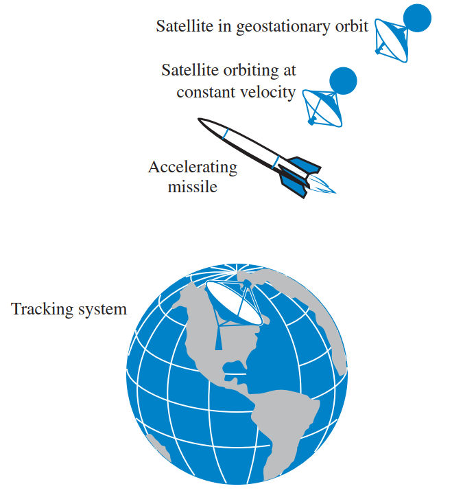
In real ECE systems:

• Antenna pointing at a satellite must not “settle” with a 5° offset.
• Robot arm placing chips on a PCB must not have a 0.5 mm final offset.
• Motor speed controller must maintain constant speed under load changes.

Steady-state error quantifies how much mismatch remains after transients die out.

Important

Key idea: Even a stable system with “nice” transients can have unacceptable steady-state error.

Use examples students know: servo motor that seems to “lock” but is just slightly off.

Contrast with stability: an unstable system never reaches steady state; steady-state error only makes sense for stable systems.

Definition of Steady-State Error

For a (stable) feedback system:

• Input: \(r(t)\)
• Output: \(c(t)\)
• Error: \(e(t) = r(t) - c(t)\)

Steady-state error:

\[ e_{ss} = e(\infty) = \lim_{t \to \infty} e(t) \]

We evaluate \(e_{ss}\) using standard test inputs that model physical motion of a position system:

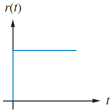
• Step: constant position
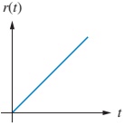
• Ramp: constant velocity
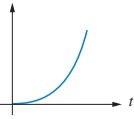
• Parabola: constant acceleration

TABLE 7.1 – Test Inputs

Name	Time function	Laplace
Step	\(1\)	\(\dfrac{1}{s}\)
Ramp	\(t\)	\(\dfrac{1}{s^2}\)
Parabola	\(\dfrac{t^2}{2}\)	\(\dfrac{1}{s^3}\)

Clarify the small correction: for a parabolic input with constant acceleration, the usual time function is \(\frac{1}{2} t^2\) with Laplace \(\frac{1}{s^3}\). The original table in the text has a typo; use the consistent version here.

Explain that for steady-state error design we care about these “idealized” inputs because: - They correspond to basic motion primitives (const position/velocity/accel). - They’re easy to handle in Laplace domain.

Visualizing the Test Inputs

Step Waveform

Step input: constant position command

Ramp Waveform

Ramp input: linearly increasing position (constant velocity target)

Parabola Waveform

Parabolic input: accelerating target (constant acceleration)

Test inputs for various targets

Use Figure 7.1 to connect to physical scenarios: - Step → holding a satellite fixed in geostationary orbit (constant angle). - Ramp → tracking a satellite moving at constant angular rate across the sky. - Parabola → tracking a missile with constant angular acceleration.

Ask: Which test input should we care about if we want to track a slowly drifting temperature? (Step or slow ramp.)

Steady-State Error Requires Stability

We focus on stable systems:

• Natural response → \(0\) as \(t \to \infty\)
• Eventually only forced response remains
• Makes sense to talk about a finite steady-state value

Unstable systems:

• Natural response grows without bound
• Output dominates input
• “Steady-state error” formulas from this chapter do not apply

Warning

Always check closed-loop stability before trusting any steady-state error calculation.

Mention Routh-Hurwitz (Chapter 6) as the usual tool.

In practice, design loop: choose architecture → check stability → then compute steady-state error. Doing it in reverse can lead to nonsense (finite error statements on unstable systems).

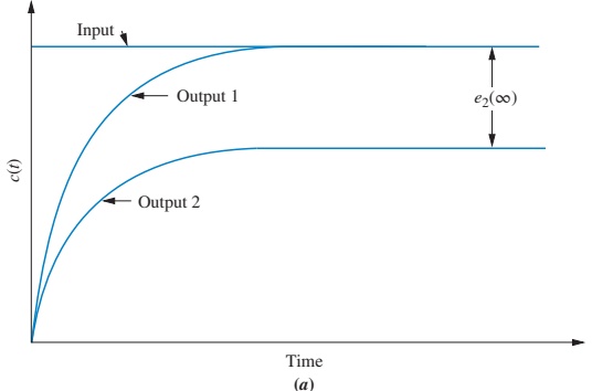
How Do We “See” Steady-State Error?

Step input and outputs

• For a step input:
  • Output 1: output converges exactly to input → \(e_{ss} = 0\)
  • Output 2: output converges to a different constant → finite \(e_{ss}\)

Ramp input and outputs

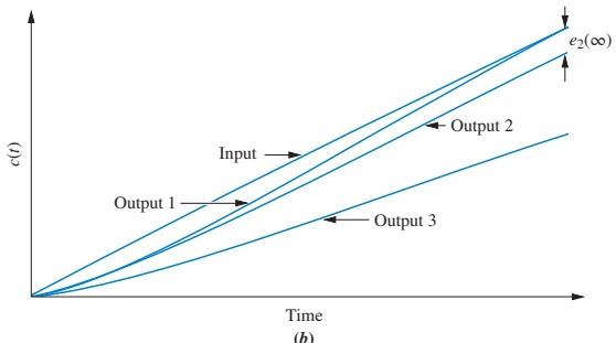
• For a ramp input:
  • Output 1: slope and offset match → \(e_{ss} = 0\)
  • Output 2: same slope, different offset → finite \(e_{ss}\)
  • Output 3: different slope → error grows without bound → \(e_{ss} = \infty\)

Emphasize: we measure error vertically between input and output after transients die out.

For the ramp case, “infinite error” means the difference grows linearly without bound.

Ask students: looking at Output 3 for the ramp, what kind of system behavior might cause this? (Not enough integrators to match input slope.)

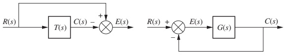
General Closed-Loop View of Error

General closed-loop system

General error representation

• Closed-loop transfer: \(T(s) = \dfrac{C(s)}{R(s)}\)
• Error: \(E(s) = R(s) - C(s)\)

Unity feedback case

Same diagram with \(H(s)=1\):

• \(E(s) = R(s) - C(s)\)
• \(C(s) = E(s) G(s)\)
• Focus in Sections 7.2–7.4: unity feedback systems

Clarify: We will first derive formulas in terms of \(T(s)\), then show a more insightful form in terms of \(G(s)\) for unity feedback.

Students often conflate \(G(s)\) and \(T(s)\); emphasize: - \(G(s)\) = forward path (controller + plant). - \(T(s)\) = closed-loop transfer from \(R\) to \(C\).

7.2 Steady-State Error in Terms of \(T(s)\)

From the general block diagram:

1. \(E(s) = R(s) - C(s)\)
2. \(C(s) = T(s) R(s)\)

So:

\[ E(s) = R(s) - T(s) R(s) = R(s) \bigl[1 - T(s)\bigr] \]

To find steady-state error: apply the final value theorem

\[ e(\infty) = \lim_{t \to \infty} e(t) = \lim_{s \to 0} s E(s) \]

Thus:

\[ e(\infty) = \lim_{s \to 0} s R(s) \bigl[1 - T(s)\bigr] \]

Tip

Use this form when \(T(s)\) is given directly and the system is known to be stable.

Remind students of final value theorem conditions:

• All poles of \(sE(s)\) in left half-plane, except possibly a simple pole at the origin.
• The closed-loop system must be stable (no RHP poles in \(T(s)\)).

Otherwise, final value theorem gives wrong answers.

Example 7.1 – Error from \(T(s)\)

Problem

Given closed-loop transfer function:

\[ T(s) = \frac{5}{s^2 + 7s + 10} \]

Find the steady-state error for a unit step input.

Solution

Step input: \(R(s) = \dfrac{1}{s}\)

1. Compute \(E(s)\):

\[ E(s) = R(s) \bigl[1 - T(s)\bigr] = \frac{1}{s} \left(1 - \frac{5}{s^2 + 7s + 10}\right) \]

Combine terms:

\[ E(s) = \frac{s^2 + 7s + 10 - 5}{s \left(s^2 + 7s + 10\right)} = \frac{s^2 + 7s + 5}{s \left(s^2 + 7s + 10\right)} \]

2. Apply final value theorem (system is stable):

\[ e(\infty) = \lim_{s \to 0} s E(s) = \lim_{s \to 0} \frac{s^2 + 7s + 5}{s^2 + 7s + 10} = \frac{5}{10} = \frac{1}{2} \]

So the steady-state error is \(e_{ss} = 0.5\).

Work slowly through the algebra on the board.

Highlight: numerator and denominator both go to constants as \(s \to 0\) → nice finite limit.

Ask: What does \(e_{ss} = 0.5\) mean physically if the input step is 1 rad? (Output settles at 0.5 rad away from input.)

7.2 Steady-State Error in Terms of \(G(s)\) (Unity Feedback)

For unity feedback:

Block diagram:

• \(C(s) = E(s) G(s)\)
• \(E(s) = R(s) - C(s)\)

Algebra:

1. \(E(s) = R(s) - C(s)\)

2. \(C(s) = E(s) G(s)\)

3. Substitute:

   \(E(s) = R(s) - E(s) G(s)\)

4. Solve for \(E(s)\):

   \[ E(s) = \frac{R(s)}{1 + G(s)} \]

Apply final value theorem:

\[ e(\infty) = \lim_{s \to 0} s E(s) = \lim_{s \to 0} \frac{s R(s)}{1 + G(s)} \]

This is our master formula for unity feedback steady-state error.

Note

This form makes it easy to see the effect of open-loop dynamics \(G(s)\) and the input type \(R(s)\) on \(e_{ss}\).

Stress that this is more insightful for design: we can reason about how many integrators we need in \(G(s)\) to get zero error for a given input.

Later, this is what feeds into “system type” and static error constants.

Step Input: Error in Terms of \(G(s)\)

For a unit step input:

• \(r(t) = u(t)\)
• \(R(s) = \dfrac{1}{s}\)

Plug into the master formula:

\[ e_{step}(\infty) = \lim_{s \to 0} \frac{s \left(\frac{1}{s}\right)}{1 + G(s)} = \frac{1}{1 + \displaystyle \lim_{s \to 0} G(s)} \]

So the key quantity is the dc gain of \(G(s)\):

\[ K_p = \lim_{s \to 0} G(s) \]

Then:

\[ e_{step}(\infty) = \frac{1}{1 + K_p} \]

Explain: “dc gain” = gain at zero frequency → constant (step) input.

Already hint at calling this \(K_p\) (position constant); formal definition comes later.

Preview: - If \(K_p = \infty\) → step error zero. - If \(K_p\) finite → step error finite. - If \(K_p = 0\) → step error = 1 (no tracking at all).

When Is Step Error Zero or Finite?

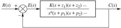
Assume

\[ G(s) = \frac{(s+z_1)(s+z_2)\cdots}{s^n (s+p_1)(s+p_2)\cdots} \]

Evaluate \(K_p = \lim_{s \to 0} G(s)\):

• If \(n = 0\) (no integrators):

  \[ K_p = \frac{z_1 z_2 \cdots}{p_1 p_2 \cdots} \quad \Rightarrow \quad \text{finite} \Rightarrow e_{step}(\infty) \text{ finite} \]

• If \(n \ge 1\) (at least one pole at origin \(\Rightarrow\) at least one integrator):

  Denominator has \(s^n\); as \(s \to 0\), denominator \(\to 0\), so

  \[ K_p = \lim_{s \to 0} G(s) = \infty \quad \Rightarrow \quad e_{step}(\infty) = 0 \]

Interpretation:

• At least one integrator in the forward path → zero step error.
• No integrator → nonzero finite step error.

Important

Integrator in the forward path eliminates constant-position error for unity feedback.

Make the time-domain connection:

• \(1/s\) factor in \(G(s)\) corresponds to \(\int\) in time.

Physical analog: a DC motor’s angle is the integral of angular velocity; thus the motor alone behaves as an integrator. That’s why simple position servos with DC motors can achieve zero static position error under unity feedback.

Ramp Input: Error in Terms of \(G(s)\)

For a unit ramp input:

• \(r(t) = t u(t)\)
• \(R(s) = \dfrac{1}{s^2}\)

From the master formula:

\[ e_{ramp}(\infty) = \lim_{s \to 0} \frac{s \left(\frac{1}{s^2}\right)}{1 + G(s)} = \lim_{s \to 0} \frac{1}{s + s G(s)} \]

If \(G(s)\) is proper and stable, for small \(s\):

• \(s \to 0 \Rightarrow s \ll s G(s)\) if \(s G(s)\) does not vanish.

So approximately:

\[ e_{ramp}(\infty) = \frac{1}{\displaystyle \lim_{s \to 0} s G(s)} = \frac{1}{K_v} \]

where

\[ K_v = \lim_{s \to 0} s G(s) \]

Explain why the simplification to \(1/(sG(s))\) is valid: for non-pathological systems, \(1 + G(s) \approx G(s)\) at low frequency when \(G(0)\) is large.

But the more rigorous path is to factor out \(s\) in denominator:

\(\frac{1}{s + s G(s)} = \frac{1}{s(1 + G(s))}\), and then use the fact that only systems with enough integrators give a nonzero finite limit.

How Many Integrators for Ramp Input?

Again, assume

\[ G(s) = \frac{(s+z_1)(s+z_2)\cdots}{s^n (s+p_1)(s+p_2)\cdots} \]

Then

\[ s G(s) = \frac{(s+z_1)(s+z_2)\cdots}{s^{n-1} (s+p_1)(s+p_2)\cdots} \]

Evaluate \(K_v = \lim_{s \to 0} s G(s)\):

• If \(n = 0\):

  \[ K_v = \lim_{s \to 0} s G(s) = 0 \Rightarrow e_{ramp}(\infty) = \infty \]

• If \(n = 1\):

  \[ K_v = \frac{z_1 z_2 \cdots}{p_1 p_2 \cdots} \quad \Rightarrow \quad \text{finite} \Rightarrow e_{ramp}(\infty) \text{ finite} \]

• If \(n \ge 2\):

  Denominator has \(s^{n-1}\) with \(n-1 \ge 1\); \(\Rightarrow\) denominator \(\to 0\) as \(s \to 0\), so

  \[ K_v = \infty \Rightarrow e_{ramp}(\infty) = 0 \]

So:

• No integrators → ramp error infinite (slopes do not match).
• One integrator → finite ramp error (same slope, offset).
• Two or more integrators → zero ramp error.

Relate to the figure with ramp outputs:

• Type 0: Output 3 (slopes differ).
• Type 1: Output 2 (same slope, constant offset).
• Type 2: Output 1 (no offset).

We’ll soon map this to formal “Type 0/1/2” terminology.

Parabolic Input: Error in Terms of \(G(s)\)

For a unit parabolic input (constant acceleration):

• \(r(t) = \dfrac{t^2}{2} u(t)\)
• \(R(s) = \dfrac{1}{s^3}\)

From the master formula:

\[ e_{parabola}(\infty) = \lim_{s \to 0} \frac{s \left(\frac{1}{s^3}\right)}{1 + G(s)} = \lim_{s \to 0} \frac{1}{s^2 + s^2 G(s)} = \frac{1}{\displaystyle \lim_{s \to 0} s^2 G(s)} = \frac{1}{K_a} \]

where

\[ K_a = \lim_{s \to 0} s^2 G(s) \]

Again use \(G(s)\) with \(n\) integrators:

\[ s^2 G(s) = \frac{(s+z_1)(s+z_2)\cdots}{s^{n-2} (s+p_1)(s+p_2)\cdots} \]

• If \(n = 0\) or \(n = 1\):

  \(s^{n-2}\) is in numerator → \(\lim s^2 G(s) = 0\) → error infinite.

• If \(n = 2\):

  \(K_a\) finite → finite parabolic error.

• If \(n \ge 3\):

  \(K_a = \infty\) → zero parabolic error.

This pattern continues: to track an input whose \(k\)-th derivative is constant, you need at least \(k+1\) integrators to get zero error.

For this course we mainly stick to step, ramp, parabolic.

Example 7.2 – System with No Integrators

System for Example 7.2

Assume closed-loop stable. There are no \(1/s\) factors in \(G(s)\).

Inputs:

1. \(5 u(t)\) → \(R(s) = \dfrac{5}{s}\)
2. \(5 t u(t)\) → \(R(s) = \dfrac{5}{s^2}\)
3. \(5 t^2 u(t)\) → \(R(s) = \dfrac{10}{s^3}\)

Given in text: \(G(s)\) has dc gain \(\lim_{s \to 0} G(s) = 20\).

1. Step input:

   \[ e_{step}(\infty) = \frac{5}{1 + \lim_{s\to 0} G(s)} = \frac{5}{1 + 20} = \frac{5}{21} \]

2. Ramp input:

   \[ e_{ramp}(\infty) = \frac{5}{\lim_{s \to 0} s G(s)} = \frac{5}{0} = \infty \]

3. Parabolic input:

   \[ e_{parabola}(\infty) = \frac{10}{\lim_{s \to 0} s^2 G(s)} = \frac{10}{0} = \infty \]

Ask the class:

• Why is ramp and parabolic error infinite? (No integrators → cannot keep up with increasing input.)
• What change to \(G(s)\) could reduce ramp error? (Add an integrator.)

We’re building toward the concept of “Type 0” here: no integrators, good for steps only.

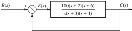
Example 7.3 – System with One Integrator

System for Example 7.3

Now \(G(s)\) includes one \(1/s\) factor (one integrator). Assume closed-loop stable.

Given in text:

• \(\lim_{s \to 0} G(s) = \infty\) (due to integrator).
• \(\lim_{s \to 0} s G(s) = 100\).

Inputs:

1. \(5 u(t)\):

   \[ e_{step}(\infty) = \frac{5}{1 + \lim_{s\to 0} G(s)} = \frac{5}{\infty} = 0 \]

2. \(5 t u(t)\):

   \[ e_{ramp}(\infty) = \frac{5}{\lim_{s \to 0} s G(s)} = \frac{5}{100} = \frac{1}{20} \]

3. \(5 t^2 u(t)\):

   \[ e_{parabola}(\infty) = \frac{10}{\lim_{s \to 0} s^2 G(s)} = \frac{10}{0} = \infty \]

So:

• Step: zero error
• Ramp: finite error
• Parabola: infinite error

Tip

Adding one integrator moved us from “good for steps only” to “steps perfect, ramps finite error”.

Relate this to system type: this is a Type 1 system.

Point out that integrators improve steady-state error performance but can hurt stability margins and transient response; trade-offs come later (root locus, design).

Skill-Assessment 7.1 – Stability First

Given:

\[ G(s) = \frac{10(s+20)(s+30)}{s (s+25)(s+35)} \]

• This has one integrator → candidate Type 1.
• Closed-loop is stable (stated in answer).

1. Find steady-state errors for inputs \(15 u(t)\), \(15 t u(t)\), \(15 t^2 u(t)\).

Text answer:

• \(e_{step}(\infty) = 0\) (Type 1 → zero step error).
• \(e_{ramp}(\infty) = 2.1875\).
• \(e_{parabola}(\infty) = \infty\).

2. For

\[ G(s) = \frac{10(s+20)(s+30)}{s^2 (s+25)(s+35)(s+50)} \]

The closed-loop system is unstable, so steady-state error formulas cannot be applied.

Highlight the message: - Always check stability. - For the second \(G(s)\), adding another integrator might improve theoretical steady-state error, but destroys stability.

This is a nice example of design trade-off.

7.3 Static Error Constants

We now formalize the three “special limits” we’ve seen:

• Step: \(e_{step}(\infty) = \dfrac{1}{1 + \displaystyle \lim_{s \to 0} G(s)}\)
• Ramp: \(e_{ramp}(\infty) = \dfrac{1}{\displaystyle \lim_{s \to 0} s G(s)}\)
• Parabola: \(e_{parabola}(\infty) = \dfrac{1}{\displaystyle \lim_{s \to 0} s^2 G(s)}\)

Define static error constants:

• Position constant:

  \[ K_p = \lim_{s \to 0} G(s) \]

• Velocity constant:

  \[ K_v = \lim_{s \to 0} s G(s) \]

• Acceleration constant:

  \[ K_a = \lim_{s \to 0} s^2 G(s) \]

Then:

• \(e_{step}(\infty) = \dfrac{1}{1 + K_p}\)
• \(e_{ramp}(\infty) = \dfrac{1}{K_v}\)
• \(e_{parabola}(\infty) = \dfrac{1}{K_a}\)

Important

Larger static error constant \(\Rightarrow\) smaller steady-state error (for the corresponding input).

Relate to transient specs: \(\zeta, \omega_n, T_s, \%OS\) specify transient performance; \(K_p, K_v, K_a\) specify steady-state performance.

Also emphasize: \(K_p, K_v, K_a\) can be 0, finite, or infinite.

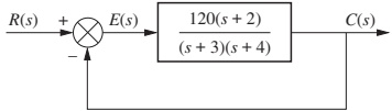
Example 7.4 – Using Static Error Constants

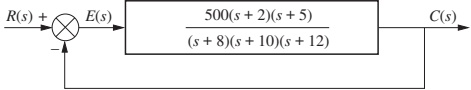
For each system in Figure 7.7, compute \(K_p, K_v, K_a\) and the corresponding steady-state error for step, ramp, and parabola.

System (a) – Type 0

System 7.7(a)

Given (from text calculations):

• \(K_p = \dfrac{500 \cdot 2 \cdot 5}{8 \cdot 10 \cdot 12} = 5.208\)
• \(K_v = 0\) (no integrator)
• \(K_a = 0\)

Hence:

• Step: \(e(\infty) = \dfrac{1}{1 + K_p} \approx 0.161\)
• Ramp: \(e(\infty) = \dfrac{1}{K_v} = \infty\)
• Parabola: \(e(\infty) = \dfrac{1}{K_a} = \infty\)

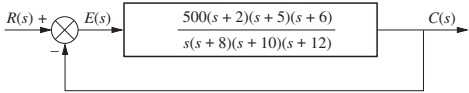
System (b) – Type 1

System 7.7(b)

• \(K_p = \infty\) (integrator present)
• \(K_v = \dfrac{500 \cdot 2 \cdot 5 \cdot 6}{8 \cdot 10 \cdot 12} = 31.25\)
• \(K_a = 0\)

Hence:

• Step: \(e(\infty) = \dfrac{1}{1 + \infty} = 0\)
• Ramp: \(e(\infty) = \dfrac{1}{K_v} = \dfrac{1}{31.25} \approx 0.032\)
• Parabola: \(e(\infty) = \dfrac{1}{0} = \infty\)

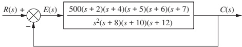
System (c) – Type 2

System 7.7(c)

• \(K_p = \infty\)
• \(K_v = \infty\)
• \(K_a = \dfrac{500 \cdot 2 \cdot 4 \cdot 5 \cdot 6 \cdot 7}{8 \cdot 10 \cdot 12} = 875\)

Hence:

• Step: \(e(\infty) = 0\)
• Ramp: \(e(\infty) = 0\)
• Parabola: \(e(\infty) = \dfrac{1}{875} \approx 1.14 \times 10^{-3}\)

Walk through one system in detail; for the others, sketch the counting argument: how many pure \(1/s\) factors? That determines which constants are finite vs. infinite.

Emphasize the pattern: increasing system type (more integrators) progressively improves steady-state error for higher-order inputs.

System Type – Formal Definition

Generic unity feedback system

Consider a unity feedback system with forward path:

\[ G(s) = \frac{(s+z_1)(s+z_2)\cdots}{s^n (s+p_1)(s+p_2)\cdots} \]

System type is defined as the number of pure integrations in the forward path, i.e., the exponent \(n\) of \(1/s\):

• \(n = 0\) → Type 0 system
• \(n = 1\) → Type 1 system
• \(n = 2\) → Type 2 system
• etc.

System type determines the pattern of static error constants and steady-state errors.

Note

In design problems, first identify system type by counting integrators in \(G(s)\) for a unity feedback configuration.

Clarify: pure integration means a pole exactly at the origin (\(1/s\)). Complex poles near the origin or real poles close to zero are not counted as integrators for system type.

Important for exam-type questions: do not confuse near-zero poles with actual integrators.

Summary Table – Input vs. Type vs. Error

TABLE 7.2 – Relationships between input, system type, static error constants, and steady-state error

Input	Error formula	Type 0	Type 0 error	Type 1	Type 1 error	Type 2	Type 2 error
Step, \(u(t)\)	\(\dfrac{1}{1+K_p}\)	\(K_p =\) finite	\(\dfrac{1}{1+K_p}\)	\(K_p = \infty\)	0	\(K_p = \infty\)	0
Ramp, \(t u(t)\)	\(\dfrac{1}{K_v}\)	\(K_v = 0\)	\(\infty\)	\(K_v =\) finite	\(\dfrac{1}{K_v}\)	\(K_v = \infty\)	0
Parabola, \(\dfrac{t^2}{2}u(t)\)	\(\dfrac{1}{K_a}\)	\(K_a = 0\)	\(\infty\)	\(K_a = 0\)	\(\infty\)	\(K_a =\) finite	\(\dfrac{1}{K_a}\)

Tip

Memorize the pattern rather than the whole table:

• Type 0: good for steps only (finite step error).
• Type 1: perfect steps, finite ramps, bad parabolas.
• Type 2: perfect steps and ramps, finite parabolas.

Use this table to quickly answer conceptual questions:

• “What is the steady-state error for a ramp input in a Type 2 system?” → 0.
• “What is \(K_v\) for a Type 0 system?” → 0.

Good to do a quick in-class quiz using multiple-choice clickers.

Skill-Assessment 7.2 – Practice with System Type

Given unity feedback:

\[ G(s) = \frac{1000 (s+8)}{(s+7)(s+9)} \]

Step 1: Find system type, \(K_p\), \(K_v\), \(K_a\).

• No factor of \(1/s\) → Type 0.
• \(K_p = \lim_{s \to 0} G(s) = \dfrac{1000 \cdot 8}{7 \cdot 9} \approx 127\).
• \(K_v = \lim_{s \to 0} s G(s) = 0\).
• \(K_a = \lim_{s \to 0} s^2 G(s) = 0\).

Step 2: Steady-state errors:

• Step:

  \[ e_{step}(\infty) = \frac{1}{1 + K_p} \approx 7.8 \times 10^{-3} \]

• Ramp:

  \[ e_{ramp}(\infty) = \frac{1}{K_v} = \infty \]

• Parabola: \(\dfrac{1}{K_a} = \infty\).

This is a realistic situation: a high-gain Type 0 plant behaves well for step inputs but poorly for velocity/acceleration tracking.

Later, using PI or PID control we can change system type “seen” by the loop.

7.4 Using Static Error Constants as Specifications

Engineers specify desired steady-state performance via \(K_p, K_v, K_a\), e.g.:

• “Design such that \(K_p = 1000\)”
• “Design a system with \(K_v = 20\)”

A specification like \(K_v = 1000\) implies:

1. System is stable.

2. System is Type 1 (only Type 1 has finite nonzero \(K_v\)).

3. The relevant test input is a ramp.

4. Steady-state error to a unit-slope ramp is

   \[ e_{ramp}(\infty) = \frac{1}{K_v} = 0.001 \]

   For a ramp with slope \(A\), error is \(\dfrac{A}{K_v}\).

Note

Just from the numeric value of \(K_p\) or \(K_v\), you can infer system type, test input, and error magnitude.

This is powerful in requirements documents: specifying a single number like \(K_v\) tells designers a lot.

Encourage students to think: if they see \(K_p\) or \(K_v\) in specs from a customer, what does it say about expected motion profile (position vs. velocity tracking)?

Example 7.5 – Interpreting \(K_p = 1000\)

Spec: \(K_p = 1000\).

This implies:

1. System is stable (otherwise \(K_p\) would be meaningless as a spec).

2. System is Type 0 (only Type 0 can have finite \(K_p\); Type 1 and above have \(K_p = \infty\)).

3. Test input is a step (position constant).

4. Steady-state error to a unit step is:

   \[ e_{step}(\infty) = \frac{1}{1 + K_p} = \frac{1}{1001} \]

So the output will be within about 0.1% of the commanded step in steady state.

Ask: Does \(K_p = 1000\) tell us anything about ramp performance? (No, for Type 0, ramp error is still infinite.)

Also note: large \(K_p\) usually means large loop gain at low frequency, which can affect stability margins.

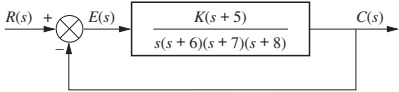
Example 7.6 – Designing Gain \(K\) from Steady-State Spec

System for Example 7.6

Problem

Given unity feedback with forward path \(G(s)\) as in figure, choose \(K\) so that there is 10% error in the steady state.

Step 1 – Identify system type and input

• From figure, forward path has one integrator → Type 1.
• Type 1: finite error only for ramp input.
• So “10% steady-state error” must refer to a ramp input.

Thus:

\[ e_{ramp}(\infty) = \frac{1}{K_v} = 0.1 \quad \Rightarrow \quad K_v = 10 \]

Step 2 – Compute \(K_v\) in terms of \(K\)

From figure’s \(G(s)\):

\[ G(s) = \frac{K \cdot 5}{s (s+6)(s+7)(s+8)} \]

Then:

\[ K_v = \lim_{s \to 0} s G(s) = \frac{K \cdot 5}{6 \cdot 7 \cdot 8} \]

Set equal to desired \(K_v\):

\[ 10 = \frac{5K}{6 \cdot 7 \cdot 8} \]

Solve:

\[ K = 10 \cdot \frac{6 \cdot 7 \cdot 8}{5} = 672 \]

Step 3 – Check stability (Routh-Hurwitz)

At \(K = 672\), closed-loop is stable (as given in text).

Warning

Meeting steady-state error specs with a large gain may degrade transient response or stability margins. Always check both.

Walk through computing \(K_v\) carefully. Students often forget to multiply by \(s\) only once, not twice.

You might show how to quickly verify closed-loop stability using Routh, but details can be deferred to a later session.

Skill-Assessment 7.3 – Gain from Ramp Error

Given unity feedback:

\[ G(s) = \frac{K (s+12)}{(s+14)(s+18)} \]

System has no integrator → Type 0 → cannot have finite ramp error.

But text’s answer says \(K = 189\) for “10% error in steady state.”

Interpreting:

• For Type 0, finite error spec must be for step input.
• So \(e_{step}(\infty) = 0.1\).

Then:

1. \(K_p = \lim_{s \to 0} G(s) = \dfrac{12K}{14 \cdot 18}\).

2. \(e_{step}(\infty) = \dfrac{1}{1 + K_p} = 0.1\).

3. Solve for \(K_p\):

   \(0.1 = \dfrac{1}{1 + K_p} \Rightarrow K_p = 9\).

4. Then:

   \[ 9 = \frac{12K}{14 \cdot 18} \Rightarrow K = 9 \cdot \frac{14 \cdot 18}{12} = 189 \]

Use this example to emphasize:

• Always determine system type first.
• Match that with which input yields finite error.
• Only then apply the appropriate formula.

If the problem statement is ambiguous, you must infer the intended input from system type and the answer.

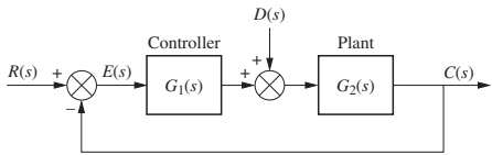
7.5 Steady-State Error Due to Disturbances

So far: we considered error due to the reference input \(R(s)\).

Now: consider disturbances \(D(s)\) entering between controller and plant.

System with disturbance

• \(G_1(s)\): controller + pre-plant dynamics
• \(G_2(s)\): plant (and maybe actuator)
• Disturbance \(D(s)\) enters between them.

We want to know how well feedback cancels the effect of \(D(s)\) on the error \(E(s)\).

Explain that in many practical systems, disturbances are loads, torque disturbances, noise, etc. For a motor, \(D(s)\) might be an external torque.

Emphasize: One major advantage of feedback is disturbance rejection.

Deriving Error with Disturbance

From the block diagram:

1. Output:

   \[ C(s) = E(s) G_1(s) G_2(s) + D(s) G_2(s) \]

2. Error:

   \[ E(s) = R(s) - C(s) \]

Substitute \(C(s)\) into error equation:

\[ E(s) = R(s) - \bigl[ E(s) G_1(s) G_2(s) + D(s) G_2(s) \bigr] \]

Solve for \(E(s)\):

\[ E(s) = \frac{1}{1 + G_1(s) G_2(s)} R(s) - \frac{G_2(s)}{1 + G_1(s) G_2(s)} D(s) \]

Apply final value theorem:

\[ \begin{aligned} e(\infty) &= \lim_{s \to 0} s E(s) \\ &= \lim_{s \to 0} \frac{s}{1 + G_1(s) G_2(s)} R(s) - \lim_{s \to 0} \frac{s G_2(s)}{1 + G_1(s) G_2(s)} D(s) \\ &= e_R(\infty) + e_D(\infty) \end{aligned} \]

Where:

• \(e_R(\infty)\): contribution from reference \(R(s)\) (already studied).
• \(e_D(\infty)\): contribution from disturbance \(D(s)\).

Highlight superposition: because the system is linear, we can treat reference and disturbance separately and add their effects.

Focus now on \(e_D(\infty)\) for a particular \(D(s)\) (step disturbance).

Step Disturbance – Expression for \(e_D(\infty)\)

Assume a step disturbance:

• \(d(t) = u(t)\)
• \(D(s) = \dfrac{1}{s}\)

The disturbance contribution to steady-state error is:

\[ e_D(\infty) = -\lim_{s \to 0} \frac{s G_2(s)}{1 + G_1(s) G_2(s)} D(s) = -\lim_{s \to 0} \frac{s G_2(s)}{1 + G_1(s) G_2(s)} \cdot \frac{1}{s} \]

Simplify:

\[ e_D(\infty) = -\lim_{s \to 0} \frac{G_2(s)}{1 + G_1(s) G_2(s)} \]

With some algebra (factor \(G_2(s)\) out of denominator), this can be rearranged as:

\[ e_D(\infty) = -\frac{1}{\displaystyle \lim_{s \to 0} \frac{1}{G_2(s)} + \lim_{s \to 0} G_1(s)} \]

Important

To reduce error from a step disturbance, either:

• Increase dc gain of controller \(G_1(s)\), or
• Decrease dc gain of plant \(G_2(s)\).

Intuition: see the next slide with the rearranged block diagram. Increasing loop gain \(G_1G_2\) makes the feedback better at rejecting disturbances.

However, decreasing \(G_2\) may not be practical if it represents physical plant gain. More often we increase \(G_1\) or add integrators in \(G_1\).

Disturbance as Input – Rearranged View

Disturbance as input

Set \(R(s) = 0\) and redraw:

• Input: disturbance \(D(s)\)
• Output: error \(E(s)\)

We can think of the block diagram as a system from \(D(s)\) to \(E(s)\).

To minimize steady-state \(E(s)\):

• Increase dc gain of \(G_1(s)\) → error is amplified and fed forward to cancel disturbance.
• Reduce dc gain of \(G_2(s)\) → disturbance effect on output smaller.

Walk through the signal flow qualitatively:

• Disturbance adds into plant input; plant output influences error through feedback.
• Over time, error adjusts so that the feedback through \(G_1\) cancels the effect of \(D(s)\) at the plant input.

Large \(G_1\) makes this cancellation more effective.

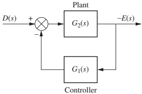
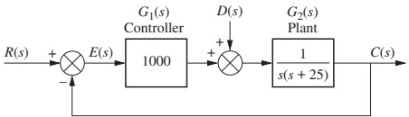
Example 7.7 – Disturbance Rejection

System for Example 7.7

Problem

Find steady-state error component due to a step disturbance for the system in the figure.

Given in text:

• System is stable.
• \(G_1(s)\) has large dc gain; \(G_2(s)\) has infinite dc gain.

Using the formula:

\[ e_D(\infty) = -\frac{1}{\displaystyle \lim_{s \to 0} \frac{1}{G_2(s)} + \lim_{s \to 0} G_1(s)} \]

Given:

• \(\lim_{s \to 0} \dfrac{1}{G_2(s)} = 0\) (since \(G_2(0) = \infty\))
• \(\lim_{s \to 0} G_1(s) = 1000\)

Then:

\[ e_D(\infty) = -\frac{1}{0 + 1000} = -\frac{1}{1000} \]

So the steady-state error caused by a unit step disturbance is \(-10^{-3}\).

Note

Error magnitude is inversely proportional to controller dc gain.

Explain sign: negative error means the controller output opposes the disturbance; but usually we care about magnitude for spec purposes.

Ask: What happens if we double the gain of \(G_1\) to 2000? Error due to disturbance halves to \(-5 \times 10^{-4}\).

But again, increasing gain indefinitely is limited by stability concerns.

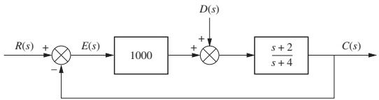
Skill-Assessment 7.4 – Disturbance Practice

System for Skill-Assessment 7.4

Given system and step disturbance \(D(s) = \dfrac{1}{s}\), evaluate disturbance-induced steady-state error.

Text answer:

\[ e_D(\infty) = -9.98 \times 10^{-4} \]

This is nearly \(-10^{-3}\), suggesting that the loop gain is around 1000 in dc.

Encourage students to compute \(\lim_{s \to 0} 1/G_2(s)\) and \(\lim_{s \to 0} G_1(s)\) for this system and verify the formula numerically as an exercise.

This reinforces use of low-frequency limits and the idea that large gain → small disturbance error.

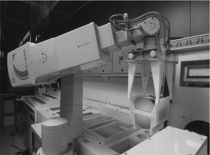
Real-World ECE Application – Robot Positioning

Robot in semiconductor manufacturing

In semiconductor manufacturing:

• Robots move wafers or chips with high precision.
• Design spec may say:
  • Step position change: final error \(< 0.01\) mm.
  • Conveyor with constant speed: tracking error \(< 0.1\) mm.

Design approach:

• Use Type 1 or Type 2 systems with appropriate \(K_p, K_v\) to meet these specs.
• Add integrators in controller (PI / PID) to increase type and improve steady-state accuracy.
• Also design for good disturbance rejection to handle load changes, friction, etc.

Remind students: the vocabulary and formulas they’re learning here translate directly into real “spec sheets” for industrial control systems.

Encourage them to read a servomotor datasheet and look for terms like “tracking error” or “steady-state accuracy”; they map to these concepts.

Summary / Key Points

1. Steady-state error \(e_{ss}\) is the difference between input and output as \(t \to \infty\).

2. It is defined for stable systems only. Always check stability.

3. Standard test inputs model motion of position systems:

   • Step (position), ramp (velocity), parabola (acceleration).

4. For unity feedback, steady-state error is conveniently computed from \(G(s)\):

   \[ e(\infty) = \lim_{s \to 0} \frac{s R(s)}{1 + G(s)} \]

5. Static error constants summarize steady-state performance:

   • \(K_p = \lim_{s \to 0} G(s)\), \(e_{step} = \dfrac{1}{1 + K_p}\).
   • \(K_v = \lim_{s \to 0} s G(s)\), \(e_{ramp} = \dfrac{1}{K_v}\).
   • \(K_a = \lim_{s \to 0} s^2 G(s)\), \(e_{parabola} = \dfrac{1}{K_a}\).

6. System type = number of integrators in \(G(s)\):

   • Type 0: finite step error; ramp/parabola errors \(\infty\).
   • Type 1: zero step error; finite ramp error; parabolic error \(\infty\).
   • Type 2: zero step and ramp error; finite parabolic error.

7. Disturbance steady-state error (for step disturbances) can be reduced by increasing controller dc gain \(G_1(0)\).

Important

Control design is a trade-off: more integrators / higher gain improve steady-state error but can harm stability and transient response.

Use this summary slide to tie together all definitions and patterns.

Before moving on in a future lecture, you might give a short conceptual quiz or a derivation exercise (e.g., show how many integrators are needed for zero error to a cubic input).

Formula Summary – Steady-State Error

General

• Error signal:

  \[ E(s) = R(s) - C(s) \]

• Closed-loop: \(C(s) = T(s) R(s)\) ⇒ \(E(s) = R(s)[1 - T(s)]\).

• Final value theorem (for stable systems):

  \[ e(\infty) = \lim_{t \to \infty} e(t) = \lim_{s \to 0} s E(s) \]

Unity Feedback (Reference Input Only)

• From open-loop \(G(s)\):

  \[ E(s) = \frac{R(s)}{1 + G(s)} \]

  \[ e(\infty) = \lim_{s \to 0} \frac{s R(s)}{1 + G(s)} \]

• Static error constants:

  \[ K_p = \lim_{s \to 0} G(s), \quad K_v = \lim_{s \to 0} s G(s), \quad K_a = \lim_{s \to 0} s^2 G(s) \]

• Steady-state errors:

  • Step \(u(t)\):

    \[ e_{step}(\infty) = \frac{1}{1 + K_p} \]

  • Ramp \(t u(t)\):

    \[ e_{ramp}(\infty) = \frac{1}{K_v} \]

  • Parabola \(\dfrac{t^2}{2} u(t)\):

    \[ e_{parabola}(\infty) = \frac{1}{K_a} \]

Disturbance Steady-State Error (Step Disturbance)

• With disturbance \(D(s)\) between \(G_1\) and \(G_2\):

  \[ e_D(\infty) = -\lim_{s \to 0} \frac{s G_2(s)}{1 + G_1(s) G_2(s)} D(s) \]

• For step \(D(s) = \dfrac{1}{s}\):

  \[ e_D(\infty) = -\frac{1}{\displaystyle \lim_{s \to 0} \frac{1}{G_2(s)} + \lim_{s \to 0} G_1(s)} \]

Encourage students to keep this slide (or a printed formula sheet) handy for homework and exams.

Point out that all formulas are just applications of: 1. Block-diagram algebra. 2. Final value theorem. 3. Low-frequency limits of \(G(s)\).

Steady-State Errors – Interactive Deck

Warm-Up: Final Value Theorem in Code

Use Python to compute

\[ e(\infty) = \lim_{s\to 0} s E(s) \]

for a given closed-loop \(T(s)\) and step input \(R(s) = 1/s\).

Edit the numerator/denominator and re-run.

Tasks:

1. Change num_T and/or den_T and see how \(e_{ss}\) changes.
2. Try to make \(e_{ss} = 0\). What condition on \(T(0)\) does that imply?

Guide students to discover: for a step, \(e_{ss} = 0\) when \(T(0) = 1\).

You can also ask them to try an unstable \(T(s)\) (e.g., with a RHP pole) and see how Sympy behaves, then remind them the final value theorem is only valid for stable systems.

Interactive: Error from Open-Loop \(G(s)\) (Unity Feedback)

Recall for unity feedback:

\[ e(\infty) = \lim_{s\to 0} \frac{s R(s)}{1 + G(s)}. \]

Below, you can define \(G(s)\) and choose the test input type.

viewof input_type = Inputs.select(
  ["step", "ramp", "parabola"],
  {label: "Input type"}
)

viewof K = Inputs.range([0, 50], {step: 1, value: 10, label: "Gain K"})

Questions:

1. For which input types do you get finite error with this \(G(s)\)?
2. How does increasing \(K\) affect the error?
3. What system type is this (Type 0, 1, or 2)? How does that match your results?

Encourage students to crank \(K\) up and notice: step error decreases but ramp and parabolic error stay infinite.

Connect to the idea: Type 0 → only step performance is improvable by gain scaling; ramp/parabola need integrators.

Exploring System Type via Integrators

Now let’s add integrators and see how system type affects \(e_{ss}\).

We define

\[ G(s) = \frac{K}{s^n (s+2)(s+3)}, \]

where n is the number of integrators → system type \(= n\).

viewof n_integrators = Inputs.range(
  [0, 3],
  {step: 1, value: 0, label: "Number of integrators n (system type)"}
)

viewof input_type2 = Inputs.select(
  ["step", "ramp", "parabola"],
  {label: "Input type"}
)

viewof K4 = Inputs.range([0, 200], {step: 10, value: 50, label: "Gain K"}
)

Try this:

1. Fix K4 = 50 and change n_integrators from 0 → 1 → 2 → 3.
2. For each input_type2, note when error becomes zero / finite / infinite.
3. Connect your observations to Table 7.2 (Type 0/1/2 behavior).

Students should rediscover:

• Type 0 (n=0): finite step error, ramp and parabola infinite.
• Type 1 (n=1): zero step, finite ramp, infinite parabola.
• Type 2 (n=2): zero step and ramp, finite parabola.

You may ask: what happens for n=3 (Type 3)? This is beyond standard table but good for deeper understanding.

Static Error Constants \(K_p, K_v, K_a\) – Interactive

We’ll compute

\[ K_p = \lim_{s\to 0} G(s),\quad K_v = \lim_{s\to 0} s G(s),\quad K_a = \lim_{s\to 0} s^2 G(s) \]

for a parameterized \(G(s)\).

Let

\[ G(s) = \frac{K(s+z)}{s^n (s+p_1)(s+p_2)}. \]

viewof n_type = Inputs.range([0, 2], {step: 1, value: 0, label: "System type n"})
viewof K3 = Inputs.range([0, 200], {step: 20, value: 100, label: "Gain K"})
viewof z = Inputs.range([0, 20], {step: 2, value: 10, label: "Zero z"})
viewof p1 = Inputs.range([1, 20], {step: 2, value: 5, label: "Pole p1"})
viewof p2 = Inputs.range([1, 20], {step: 2, value: 7, label: "Pole p2"})

Questions:

1. For each n_type, which of \(K_p, K_v, K_a\) is zero, finite, or infinite?
2. How does changing z, p1, p2 affect the finite constants?
3. For your chosen parameters, what are \(e_{step}, e_{ramp}, e_{parabola}\)?

Have students relate these computed constants to the error formulas: - \(e_{step} = 1/(1+K_p)\) - \(e_{ramp} = 1/K_v\) - \(e_{parabola} = 1/K_a\)

They should see that zeros and finite poles change magnitudes but not which errors are zero vs. infinite—that’s set by integrators.

Visualizing Step Response vs. \(K_p\) (Simple Approximation)

We’ll approximate steady-state behavior by evaluating \(T(0)\) for a step, where

\[ T(s) = \frac{G(s)}{1 + G(s)}. \]

If the input step amplitude is 1, then steady-state output ≈ \(T(0)\), and

\[ e_{ss} \approx 1 - T(0). \]

viewof K_step = Inputs.range([0, 200], {step: 10, value: 20, label: "Gain K"})

Try:

• Increase K_step. How do \(T(0)\) and \(e_{ss}\) change?
• Interpret \(T(0)\) physically (gain from input to output for DC).

Explain that for step inputs, the static gain \(T(0)\) essentially tells us how close the output gets to the commanded value in steady state.

For unity gain tracking, we want \(T(0) \approx 1\), which means high \(K_p\).

Ramp Tracking – Simulated Output and Error

Let’s simulate time-domain response to a ramp input for a Type 0 vs Type 1 system and visualize steady-state error.

We’ll use a simple numerical approximation here.

viewof K_ramp = Inputs.range([0, 100], {step: 10, value: 20, label: "Gain K"})
viewof has_integrator = Inputs.checkbox(
  ["Include integrator"],
  {label: "Include integrator in G(s)?", value: []}
)

Questions:

1. With no integrator (Type 0), does the error seem to grow without bound?
2. With an integrator (Type 1), does the error approach a finite constant?
3. How does increasing K_ramp affect the ramp error for Type 1?

This gives students a direct visual confirmation of the qualitative step–ramp–parabola behavior discussed in theory.

Emphasize the difference between ever-growing error (Type 0) vs. converging offset (Type 1).

Disturbance Rejection – Static Formula Exploration

For a disturbance entering between \(G_1\) and \(G_2\), for a step disturbance \(D(s) = 1/s\),

\[ e_D(\infty) = -\frac{1}{\displaystyle \lim_{s\to 0} \frac{1}{G_2(s)} + \lim_{s\to 0} G_1(s)}. \]

Here we’ll assume

\[ G_1(s) \approx K_1, \quad G_2(s) \approx K_2 \]

around DC, and compute \(e_D(\infty)\) interactively.

viewof K1 = Inputs.range([0, 2000], {step: 100, value: 500, label: "Controller DC gain K1 ≈ G1(0)"})
viewof K2 = Inputs.range([0.1, 10], {step: 0.1, value: 2, label: "Plant DC gain K2 ≈ G2(0)"})

Explore:

1. Increase K1 while keeping K2 fixed. What happens to eD?
2. Decrease K2 (weaker plant gain). How does that affect eD?
3. Relate to the block diagram interpretation: why does high controller gain improve disturbance rejection?

Remind students that this is a simplified dc analysis, but the trend is accurate: higher loop gain → better disturbance suppression (at low frequency).

Relate to Example 7.7 and Skill-Assessment 7.4, where \(e_D(\infty)\) was around \(-10^{-3}\).

Disturbance Rejection – Time-Domain Simulation

Now let’s simulate a disturbance step entering the plant input and see how the output error behaves.

We consider the canonical structure:

\[ G_1(s) = K_1, \quad G_2(s) = \frac{K_2}{s+1}. \]

viewof K1_d = Inputs.range([0, 1000], {step: 100, value: 500, label: "K1 (controller gain)"})
viewof K2_d = Inputs.range([0, 10], {step: 1, value: 5, label: "K2 (plant gain)"})

Try:

1. Increase K1_d. Does steady-state error magnitude decrease?
2. Change K2_d. How does that affect the shape and final value of E(t)?
3. Compare with the static formula you just explored.

This reinforces the connection between the analytic formula for \(e_D(\infty)\) and time-domain simulation.

Good to ask students: is there any trade-off in transient behavior as K1 grows large (e.g., overshoot, oscillations)? That bridges to stability and transient design topics.

Challenge: Design \(K\) for a Desired Ramp Error

Suppose you have unity feedback with

\[ G(s) = \frac{K}{s (s+2)(s+3)}, \]

which is Type 1.

You want a 10% error for a unit ramp input, i.e.,

\[ e_{ramp}(\infty) = 0.1. \]

Use the interactive code below to:

1. Compute \(K_v = \lim_{s\to 0} s G(s)\).
2. Solve for \(K\) such that \(1/K_v = 0.1\).
3. Verify with a numerical simulation of a ramp response.

Now plug that \(K\) into the previous ramp simulation slide by editing G(s) there to match this form and see if the final error matches \(\approx 0.1\).

This slide encourages students to combine symbolic manipulation (Kv derivation), numerical solving (for K), and simulation (to check).

Make sure to walk through at least once in class so students see the full loop.

Reflection – What Did You Observe?

Use this slide as a checklist:

• How does the number of integrators (system type) influence which inputs have zero / finite / infinite error?
• How does increasing gain \(K\) change steady-state error for:
  • Type 0 system with step input?
  • Type 1 system with ramp input?
• How do the static error constants \(K_p, K_v, K_a\) help you quickly predict error behavior?
• How does increasing controller dc gain help with disturbance rejection?

Consider writing down:

1. One experiment that surprised you.
2. One pattern you discovered yourself while playing with the sliders.

Encourage students to take screenshots or notes from configurations they find insightful.

You can also assign a short lab report where they must document a few parameter sweeps and interpret the results.