Reduction of Multiple Subsystems

Control 5

Imron Rosyadi

Reduction of Multiple Subsystems

Block Diagrams, Signal-Flow Graphs, and Mason’s Rule

Learning Objectives

After this session, you will be able to:

• Reduce a multi-block diagram into a single transfer function using block diagram algebra.
• Recognize and use the cascade, parallel, and feedback interconnection forms.
• Use block moves (across summing junctions and pickoff points) to reveal familiar forms.
• Convert block diagrams ↔︎ signal‑flow graphs.
• Compute a system transfer function using Mason’s Rule.
• Analyze and design second‑order feedback systems built from multiple subsystems (overshoot, settling time, etc.).

Clarify: This lecture will not cover all later subsections in full state-space detail (5.7–5.8), but we build the foundation:

• Block diagrams (5.2)
• Feedback analysis & design (5.3)
• Signal-flow graphs (5.4)
• Mason’s Rule (5.5)

Point out that these are heavily used in later state-space sections.

5.1 Why Reduce Multiple Subsystems?

We start with subsystems:

• Each subsystem: a block with input, output, and transfer function.
• Real systems: many subsystems interconnected.

Goal:

• Replace the whole interconnection by one equivalent transfer function from input to output.
• Then we can:
  • Apply transient-analysis formulas.
  • Study stability (poles).
  • Design gains and compensators.

Block diagrams vs. signal-flow graphs

• Block diagrams
  • Blocks + summing junctions + pickoff points.
  • Common in frequency-domain analysis & design.
• Signal‑flow graphs
  • Nodes = signals.
  • Directed branches = transfer functions.
  • Very convenient for state‑space and for using Mason’s Rule.

FIGURE 5.1 – The space shuttle: countless subsystems, many of them control systems.

Use the shuttle image to prompt a quick discussion:

• Ask: “Which subsystems are control systems?” (examples: attitude control, engine thrust control, environmental control, power management, navigation, etc.)

Then emphasize: each of those high-level control systems is itself formed from many smaller subsystems (sensors, filters, compensators, actuators). We need systematic ways to model their interconnections.

Block Diagram Elements (LTI Systems)

All basic block diagram components:

FIGURE 5.2 – Components of a block diagram for a linear, time‑invariant system.

• Blocks: systems / subsystems with transfer function.
• Summing junctions: algebraic sum of inputs.
• Pickoff points: copy a signal undiminished to multiple locations.

Walk through Figure 5.2:

• 1. typical block: system with transfer function G(s).
• 2. typical input/output labeling.
• 3. summing junction: show that \(C(s) = R_1(s) \pm R_2(s) \pm R_3(s)\). Stress that signs matter.
• 4. pickoff: signal fan-out, no attenuation.

Highlight assumption: signals are unloaded unless we explicitly include loading through transfer functions. This is important in the cascade loading example later.

5.2 Basic Interconnection Forms

We focus on three fundamental interconnections:

1. Cascade (series)
2. Parallel
3. Feedback

Every complicated block diagram can be reduced by repeatedly:

• Recognizing pieces in one of these forms.
• Replacing that piece with its equivalent single block.

Note

If you can reduce cascade, parallel, and feedback, and you know how to move blocks, you can handle almost any linear block diagram.

Remind students that these are the “algebra rules” of block diagrams. Just like simplifying algebraic expressions, you apply patterns repeatedly.

Tell them they will use these patterns constantly in exam problems and in design work.

Cascade Form – Concept

Cascaded subsystems:

FIGURE 5.3 – (a) Cascaded subsystems; (b) equivalent transfer function.

Given:

• Subsystems \(G_1(s), G_2(s), G_3(s)\) in series.

Equivalent transfer function:

\[ G_e(s) = G_3(s)\,G_2(s)\,G_1(s) \]

(assuming no loading between stages).

Analogy (ECE hardware):

• Series of gain stages in an amplifier chain.
• A digital filter realized as cascaded biquad sections.

Derive quickly:

• Let input be \(R(s)\).
• After \(G_1\): \(X_1(s) = G_1(s)R(s)\).
• After \(G_2\): \(X_2(s) = G_2(s)X_1(s) = G_2(s)G_1(s)R(s)\).
• After \(G_3\): \(C(s) = G_3(s)X_2(s) = G_3(s)G_2(s)G_1(s)R(s)\).
• So \(C/R = G_3 G_2 G_1\).

Stress that this is correct if stages don’t “electrically load” each other (i.e., the representation as independent transfer functions is valid).

Cascade Form – When Loading Breaks It

RC networks illustrate loading:

FIGURE 5.4 – Loading in cascaded systems.

FIGURE 5.4 – Loading in cascaded systems.

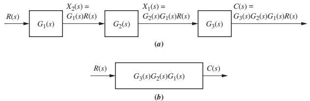
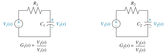
For each isolated network:

• First RC: \[ G_1(s) = \frac{V_1(s)}{V_i(s)} = \frac{\frac{1}{R_1 C_1}}{s + \frac{1}{R_1 C_1}} \]

• Second RC: \[ G_2(s) = \frac{V_2(s)}{V_1(s)} = \frac{\frac{1}{R_2 C_2}}{s + \frac{1}{R_2 C_2}} \]

If we naively cascade:

\[ G_{\text{naive}}(s) = G_2(s)G_1(s) = \frac{\frac{1}{R_1 C_1 R_2 C_2}}{s^2 + \left(\frac{1}{R_1 C_1} + \frac{1}{R_2 C_2}\right)s + \frac{1}{R_1 C_1 R_2 C_2}} \]

But the true transfer function (from circuit analysis) is:

\[ G(s) = \frac{V_2(s)}{V_i(s)} = \frac{\frac{1}{R_1 C_1 R_2 C_2}}{s^2 + \left(\frac{1}{R_1 C_1} + \frac{1}{R_2 C_2} + \frac{1}{R_2 C_1}\right)s + \frac{1}{R_1 C_1 R_2 C_2}} \]

They are not equal: extra term \(\frac{1}{R_2 C_1}\) appears due to loading.

Important

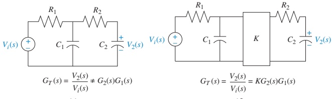
Block diagram algebra assumes no loading between blocks. If electrical loading exists, you must include it in the model.

Explain physically:

• The first RC’s output sees the input impedance of the second RC, altering its dynamics.
• The independent transfer-function model for each block is only valid if their connection doesn’t change their behavior (e.g., buffered interfaces).

Then point to Figure 5.4(d): show that adding an amplifier/buffer isolates the stages.

Conclusion: in control block diagrams, we assume signals are ideal, so cascade multiplication is valid. But as hardware designers, we must check that assumption.

Preventing Loading – Buffering

RC networks with amplifier buffer

• Amplifier/buffer between RC networks:
  • High input impedance ⇒ does not load previous stage.
  • Low output impedance ⇒ drives next stage like an ideal source.

Then:

\[ G_{\text{eq}}(s) = K\,G_2(s)G_1(s) \]

where \(K\) is the amplifier gain.

Connect to op-amp circuits:

• A voltage follower (unity-gain buffer) prevents loading and preserves the cascade product.

Tie back to block diagrams: when we draw multiple blocks in cascade, we implicitly assume we have such ideal buffering (or non-interacting signals).

Parallel Form

FIGURE 5.5(a) – Parallel subsystems.

FIGURE 5.5(b) – Equivalent transfer function.

Parallel subsystems:

• Same input goes to each block.
• Outputs are algebraically summed.

Equivalent transfer function:

\[ G_e(s) = \pm G_1(s) \pm G_2(s) \pm G_3(s) \]

(plus/minus depending on summing junction signs).

Real ECE example:

• Two sensor paths (e.g., high‑frequency and low‑frequency channels) summed to form one control input.

Demonstrate quickly: Suppose input is \(R(s)\). Then:

• \(C_1 = G_1 R\)
• \(C_2 = G_2 R\)
• \(C_3 = G_3 R\) Total output \(C = \pm C_1 \pm C_2 \pm C_3 = (\pm G_1 \pm G_2 \pm G_3)R\). So \(C/R = G_e(s)\).

Point out that parallel is often used for implementing sums/differences of dynamics, e.g., PD = sK_d + K_p = sK_d in parallel with K_p.

Feedback Form – The Core Control Topology

Typical feedback control system:

Feedback system and simplified model

Simplified feedback model

Equivalent feedback transfer function

FIGURE 5.6 – (a) Complete feedback system, (b) simplified, (c) equivalent transfer function.

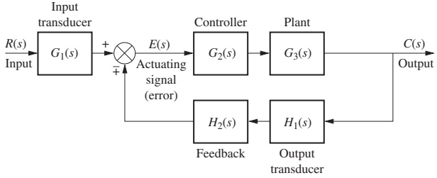
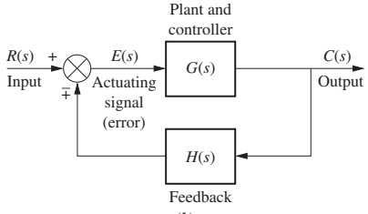
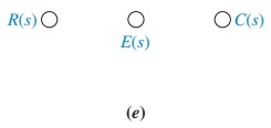
From simplified model:

• Error: \[ E(s) = R(s) \mp C(s)H(s) \]

• Output: \[ C(s) = G(s)E(s) \]

Eliminate \(E(s)\):

\[ E(s) = \frac{C(s)}{G(s)} \]

Substitute:

\[ \frac{C(s)}{G(s)} = R(s) \mp C(s)H(s) \]

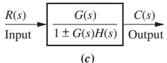
Solve for \(C(s)/R(s)\):

\[ G_e(s) = \frac{C(s)}{R(s)} = \frac{G(s)}{1 \pm G(s)H(s)} \]

The product \(G(s)H(s)\) is the open-loop transfer function or loop gain.

Derive this algebra carefully on the board so students can follow each step.

Stress sign convention:

• Minus in the denominator for negative feedback: \(G/(1+GH)\).
• Plus for positive feedback: \(G/(1-GH)\).

Real-world example: position control:

• \(G(s)\) = motor + gears + amplifier.
• \(H(s)\) = sensor scale (e.g., potentiometer).

Negative feedback drives error to zero (tracking, disturbance rejection).

Moving Blocks – Why It Matters

Complex diagrams rarely show clean cascade/parallel/feedback chunks.

We must move blocks across:

• Summing junctions
• Pickoff points

…to expose:

• Pure cascade segments
• Pure parallel segments
• Standard feedback loops

Key idea:

• You may rearrange a block diagram as long as the input–output relationship remains identical.

Warning

If you move a block incorrectly, you change the system. Always verify equivalence by writing expressions for intermediate signals.

This is like algebraic manipulation: \((a+b)c = ac+bc\). You can move c across the sum; same value, different representation.

In block diagrams: we shift transfer functions across summing junctions or pickoffs while maintaining the equality of all node signals.

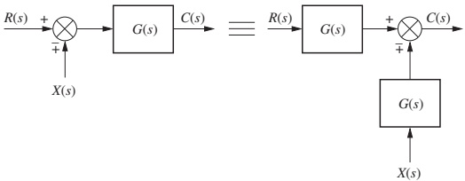
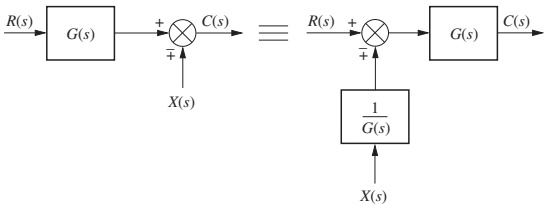
Moving Blocks Across Summing Junctions

FIGURE 5.7 – Equivalent forms for moving a block across a summing junction.

FIGURE 5.7 – Equivalent forms for moving a block across a summing junction.

• Figure 5.7(a): moving G(s) left across a summing junction that feeds it.
• Figure 5.7(b): moving G(s) right across a summing junction.

In both cases, verify:

• If both \(R(s)\) and \(X(s)\) are multiplied by \(G(s)\) before contributing to the output, the two diagrams are equivalent.

Mathematically, for 5.7(a):

\[ C(s) = [R(s) \mp X(s)]\,G(s) = R(s)G(s) \mp X(s)G(s) \]

Same result for the rearranged diagram.

Spend a minute explicitly tracing one of them:

• Start with original: \(C = G(R \mp X)\).
• After move: \(C = GR \mp GX\).

They’re equal; hence diagrams are equivalent.

Emphasize: This property is what lets us “pull” gain into or out of a feedback loop, or re-attach blocks to new nodes.

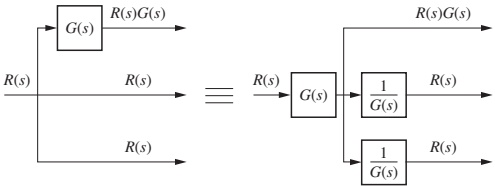
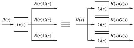
Moving Blocks Across Pickoff Points

FIGURE 5.8 – Equivalent forms for moving a block across a pickoff point.

FIGURE 5.8 – Equivalent forms for moving a block across a pickoff point.

• Move block before or after the pickoff, if:
  • All branches from the pickoff see the appropriate transformation.

Example reasoning:

• If output branches need the same scaled signal \(G(s)R(s)\), you can move \(G(s)\) before the pickoff.
• If only one branch needs scaling, \(G(s)\) must stay on that branch.

Point out a common student mistake: moving a transfer function in a way that changes which paths it affects.

Encourage them to: 1. Label key signals before and after the move. 2. Write equations to confirm equivalence.

These block-move rules are extremely useful in multi-loop diagrams.

Example 5.1 – Block Diagram Reduction via Familiar Forms

Problem: Reduce the block diagram in Figure 5.9 to a single transfer function.

FIGURE 5.9 – Block diagram for Example 5.1.

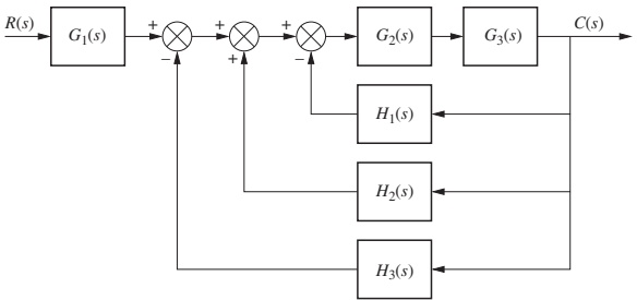
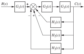
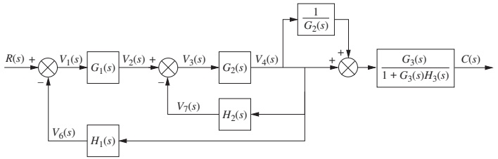
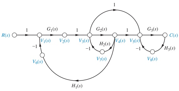
Example 5.1 – Step 1: Collapse Summing Junctions

FIGURE 5.10(a) – Collapsing three summing junctions into one.

• Multiple summing junctions in series can be combined into one junction whose inputs are the algebraic sum of all original inputs.

Explain that summing junctions are associative and commutative (like normal addition). Collapsing them does not alter the system as long as signs are preserved.

This simplifies the picture so you can more easily spot parallel/feedback relationships.

Example 5.1 – Step 2: Cascade and Parallel Recognition

FIGURE 5.10(b) – Cascade in forward path, parallel in feedback path.

Recognize:

• Forward path: \(G_2(s)\) and \(G_3(s)\) in cascade: \[ G_{\text{forward}}(s) = G_3(s)G_2(s) \]

• Feedback path: \(H_1(s), H_2(s), H_3(s)\) in parallel: \[ H_{\text{eq}}(s) = H_1(s) - H_2(s) + H_3(s) \]

Stress the skill: recognizing forms. Students often get stuck simply because they don’t see that three blocks are in parallel or cascade.

Once recognized, you quickly replace them by their equivalents, drastically simplifying the diagram.

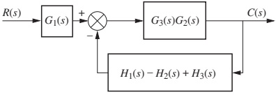
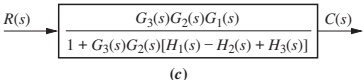
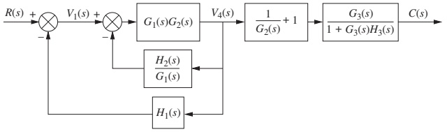
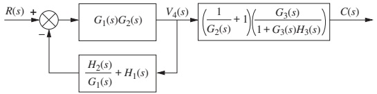
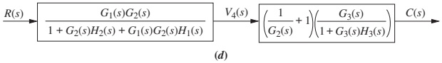
Example 5.1 – Step 3: Final Reduction

FIGURE 5.10(c) – Equivalent feedback system with cascaded \(G_1(s)\).

• Overall feedback loop: forward path \(G_3 G_2\), feedback \(H_{\text{eq}}\).

Closed-loop equivalent:

\[ \text{Inner loop:}\quad G_{\text{CL}}(s) = \frac{G_3(s)G_2(s)}{1 + G_3(s)G_2(s)\,H_{\text{eq}}(s)} \]

Then cascade with \(G_1(s)\):

\[ T(s) = \frac{C(s)}{R(s)} = G_1(s) \cdot G_{\text{CL}}(s) \]

Walk through the logic: 1. Reduce parallel feedback path to one \(H_{\text{eq}}\). 2. Apply feedback formula for inner loop. 3. Multiply by \(G_1\) in cascade.

Encourage students to write the final explicit expression if time permits.

Example 5.2 – Block Diagram Reduction by Moving Blocks

Problem: Reduce the system in Figure 5.11 to a single transfer function.

FIGURE 5.11 – Block diagram for Example 5.2.

This diagram is too tangled to reduce directly. We will:

1. Move blocks across pickoffs.
2. Create parallel pairs and simpler feedback loops.
3. Successively apply cascade/parallel/feedback reductions.

Mention that this example is intentionally more complicated to illustrate the power of block moves.

Remind students not to memorize these particular steps, but to understand the strategy: make the diagram look like known forms.

Example 5.2 – Reduction Steps (Visual Walkthrough)

We only sketch the key steps; the textbook has full details.

1. Move \(G_2(s)\) left past the pickoff; reduce the feedback loop with \(G_3(s)\) and \(H_3(s)\).

Step (a)

2. Reduce parallel pair \(1/G_2(s)\) and unity; move \(G_1(s)\) right past summing junction.

Step (b)

3. Collapse summing junctions, combine cascaded blocks, and sum feedback paths.

Step (c)

4. Apply feedback formula to get:

Step (d)

5. Final cascade multiplication yields the single equivalent transfer function:

Step (e)

FIGURE 5.12 – Steps in the block diagram reduction for Example 5.2.

As you show each figure:

• Briefly describe which rule was used (move across pickoff, reduce parallel, collapse sums, etc.).
• Encourage students to mark up their book as they follow the transformation.

If time allows, ask them to identify where negative signs would appear if any blocks were subtracted instead of added in feedback.

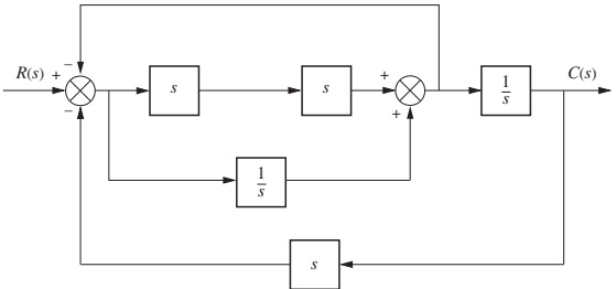
Skill-Assessment Exercise 5.1 (Concept Check)

Problem: Find equivalent transfer function \(T(s) = C(s)/R(s)\) for the system in Figure 5.13.

FIGURE 5.13 – Block diagram for Skill-Assessment Exercise 5.1.

Given answer:

\[ T(s) = \frac{s^{3} + 1}{2s^{4} + s^{2} + 2s} \]

Tip

Use this as a self-check:

• Try to re-derive \(T(s)\) by systematically using cascade, parallel, and feedback reductions.
• Compare your expression with the given result.

You don’t need to derive it fully in class (time-consuming), but you can ask:

• “What’s the first reduction step you would take?”
• “Where is the main feedback loop?”

Point them to the online full solution for practice.

5.3 Feedback Systems – From Structure to Transient Specs

Immediate application:

• Systems that reduce to second-order closed-loop forms.
• Use classic formulas for:
  • Percent overshoot (%OS)
  • Settling time \(T_s\)
  • Peak time \(T_p\)
  • Rise time \(T_r\)

Consider system:

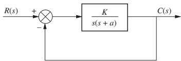
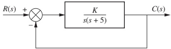
FIGURE 5.14 – Second-order feedback control system.

Closed-loop transfer function:

\[ T(s) = \frac{K}{s^{2} + a s + K} \]

Here:

• \(K\): overall gain (e.g., amplifier gain).
• \(a\): coefficient related to damping (e.g., friction, resistance).

Show how Eq. (5.9) gives this:

• Forward path: \(G(s) = \dfrac{K}{s(s+a)}\).
• Feedback: unity.
• Then \(T(s) = \dfrac{G(s)}{1 + G(s)} = \dfrac{K}{s^2+as+K}\).

Highlight: This looks exactly like the standard second-order denominator: \(s^2 + 2\zeta\omega_n s + \omega_n^2\).

So we can identify: \(\omega_n^2 = K\), \(2\zeta\omega_n = a\).

Pole Locations vs. Gain K

Poles of closed-loop system:

• For \(0 < K < a^2/4\): real, distinct (overdamped). \[ s_{1,2} = -\frac{a}{2} \pm \frac{\sqrt{a^{2} - 4K}}{2} \]

• For \(K = a^2/4\): real, equal (critically damped).

• For \(K > a^2/4\): complex conjugate (underdamped). \[ s_{1,2} = -\frac{a}{2} \pm j\frac{\sqrt{4K - a^{2}}}{2} \]

For underdamped case:

• Real part fixed at \(-a/2\).
• Imaginary part increases with \(K\).
• Implications:
  • Peak time \(T_p\) decreases (faster oscillations).
  • Percent overshoot increases (more oscillatory).
  • Settling time roughly constant (since real part fixed).

Important

Gain \(K\) trades off speed vs. overshoot. Design is about choosing \(K\) to satisfy both.

Relate to root locus intuition: as \(K\) increases, the closed-loop poles move along a locus; their real and imaginary parts control transient response.

Mention this is a simple “family” of systems parameterized by K—ideal for introducing design.

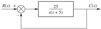
Example 5.3 – Finding Transient Response

Problem: For system in Figure 5.15, find \(T_p\), %OS, and \(T_s\).

Feedback system Example 5.3

Closed-loop transfer function:

\[ T(s) = \frac{25}{s^{2} + 5s + 25} \]

Compare with standard 2nd-order form:

\[ T(s) = \frac{\omega_n^{2}}{s^{2} + 2\zeta\omega_n s + \omega_n^{2}} \]

Identify:

• \(\omega_n^2 = 25 \Rightarrow \omega_n = 5\).
• \(2\zeta \omega_n = 5 \Rightarrow 2\zeta(5) = 5 \Rightarrow \zeta = 0.5\).

Now apply standard formulas:

• Peak time \[ T_p = \frac{\pi}{\omega_n \sqrt{1-\zeta^{2}}} = 0.726 \text{ s} \]

• Percent overshoot \[ \%OS = e^{-\zeta\pi/\sqrt{1-\zeta^{2}}} \times 100 = 16.3\% \]

• Settling time (2% criterion) \[ T_s = \frac{4}{\zeta\omega_n} = 1.6 \text{ s} \]

Reinforce the mapping:

• Denominator coefficients give \(\zeta, \omega_n\).
• Those give transient specs.

Mention that MATLAB can compute these automatically (e.g., with stepinfo), but understanding the formulas gives physical intuition.

Example 5.4 – Gain Design for Transient Response

Problem: For system in Figure 5.16, choose gain \(K\) so that step response has 10% overshoot.

FIGURE 5.16 – Feedback system for Example 5.4.

Closed-loop transfer function:

\[ T(s) = \frac{K}{s^{2} + 5s + K} \]

Identify standard form:

• \(\omega_n^2 = K \Rightarrow \omega_n = \sqrt{K}\)
• \(2\zeta\omega_n = 5 \Rightarrow 2\zeta\sqrt{K} = 5 \Rightarrow \zeta = \dfrac{5}{2\sqrt{K}}\)

Percent overshoot depends only on \(\zeta\):

\[ \%OS = e^{-\zeta\pi/\sqrt{1-\zeta^{2}}}\times 100 \]

For \(\%OS = 10\%\), from standard tables or solving numerically: \(\zeta \approx 0.591\).

Set \(\zeta = 5/(2\sqrt{K}) = 0.591\):

\[ \sqrt{K} = \frac{5}{2\zeta} \approx \frac{5}{2 \times 0.591} \approx 2.667 \]

\[ K \approx 2.667^2 \approx 17.9 \]

So design result:

• Gain \(K \approx 17.9\) gives 10% overshoot.

Tip

This is a typical design workflow: Desired %OS → \(\zeta\) → \(K\) from the denominator coefficients.

Highlight that this is design not just analysis: we solved backwards from a performance specification.

Mention that in more complex systems (higher order, zeros), the mapping isn’t so direct, and we need root locus, Bode, etc., but this gives a powerful intuition.

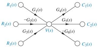
5.4 Signal-Flow Graphs – Another Representation

Key differences from block diagrams:

• Only nodes and directed branches:
  • Node = signal.
  • Branch = system/transfer function.
• Summation is implicit at each node:
  • Node value = algebraic sum of incoming signals.

FIGURE 5.17 – (a) Branch representing a system, (b) node representing a signal

FIGURE 5.17 – (c) interconnection example.

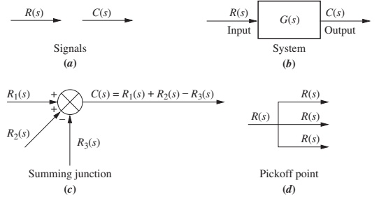
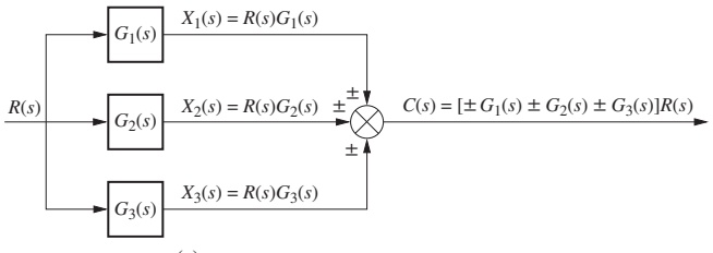
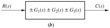
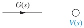
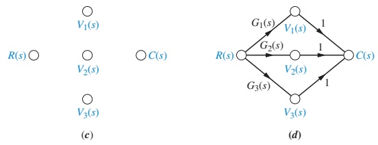
Example node equation from Figure 5.17(c):

\[ V(s) = R_1(s)G_1(s) - R_2(s)G_2(s) + R_3(s)G_3(s) \]

Note: negative input is modeled by negative branch gain (e.g., \(-G_2(s)\)), not by a separate summing junction.

Note

Signal-flow graphs are especially convenient:

• For state‑space (each state is a node).
• For using Mason’s Rule to find transfer functions.

Explain why signal-flow graphs can be more compact than block diagrams:

• No explicit summing junctions or pickoffs.
• Direct representation of equations.

Connect to state-space: each state variable x_i(t) becomes a node; its derivative equation determines incoming branches.

From Block Diagrams to Signal-Flow Graphs

Example 5.5: Convert basic block forms (cascade, parallel, feedback) into signal-flow graphs.

Strategy:

1. Draw signal nodes for each intermediate signal.
2. Connect nodes with directed branches labeled by transfer functions.
3. Use negative gains for negative feedback or subtraction.

Cascade nodes and graph

Parallel nodes and graph

Feedback nodes and graph

Feedback signal-flow graph

FIGURE 5.18 – Building signal-flow graphs for cascade, parallel, and feedback forms.

For each configuration:

• Draw R, intermediate nodes, C.
• Add arrows with G’s and H’s.
• Show how negative feedback loop is a branch from C back to the error node with gain \(-H\).

Emphasize that once you’re comfortable switching representations, you can choose whichever is more convenient for analysis.

Example 5.6 – Complex Block Diagram → Signal-Flow Graph

Convert Figure 5.11 (from Example 5.2) into a signal-flow graph.

1. Draw all signal nodes \(V_1(s), V_2(s), \dots\) etc.

Signal nodes

2. Connect them with branch gains \(G_i(s), H_i(s)\), including negative gains where appropriate.

Full signal-flow graph

3. Optionally, simplify by removing nodes that only have one incoming and one outgoing branch (series combination).

Simplified signal-flow graph

FIGURE 5.19 – Signal-flow graph development from Figure 5.11.

Explain that nodes like \(V_2, V_6, V_7, V_8\) with single in and single out can be merged by multiplying branch gains. This is akin to series combination of transfer functions.

This simplification is often done before applying Mason’s Rule to keep the bookkeeping manageable.

5.5 Mason’s Rule – Transfer Function from a Signal-Flow Graph

Mason’s Rule gives the transfer function \(C(s)/R(s)\) directly from a signal-flow graph:

\[ G(s) = \frac{C(s)}{R(s)} = \frac{\displaystyle\sum_{k} T_k \Delta_k}{\Delta} \]

Where:

• \(T_k\): the k‑th forward-path gain from input node to output node.

• \(\Delta\): the overall determinant of the graph, defined by:

  \[ \Delta = 1 - \sum (\text{individual loop gains}) + \sum (\text{products of loop gains in all nontouching loop pairs}) - \sum (\text{products of loop gains in all nontouching triplets}) + \dots \]

• \(\Delta_k\): same as \(\Delta\), but excluding all loops that touch the k-th forward path.

Key definitions:

• Loop: a path that starts and ends at the same node without visiting any node more than once.
• Loop gain: product of branch gains around a loop.
• Nontouching loops: loops that share no nodes in common.

Caution

The hardest parts of Mason’s Rule are:

1. Enumerating all loops.
2. Correctly identifying nontouching loop combinations.

Reassure students: Mason’s Rule looks intimidating, but in many practical systems:

• There are few loops.
• Often no nontouching loops.

In such cases, \(\Delta = 1 - (\text{sum of loops})\) and \(\Delta_k = 1\) or something simple.

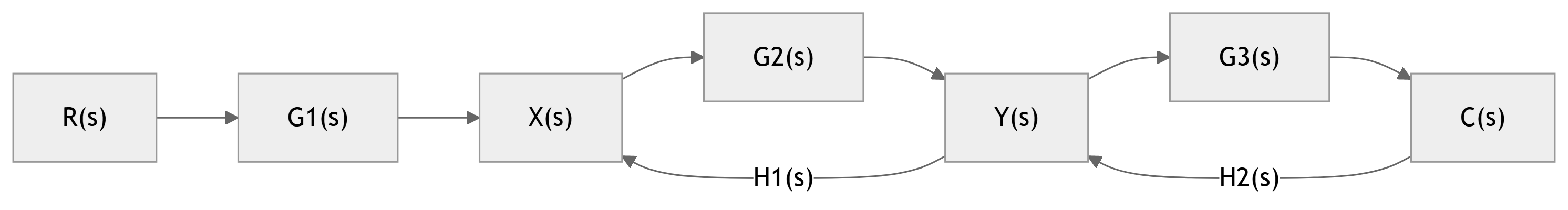
Visualizing Loops and Forward Paths

• Forward path: \(R \to G_1 \to G_2 \to G_3 \to C\).
• Loops:
  • Around \(X\) and \(Y\) via \(H_1(s)\).
  • Around \(Y\) and \(C\) via \(H_2(s)\).

Use this simple structure to practice identifying loops and nontouching loops.

This is just a self-made example for teaching. Use it to:

• Ask students: identify the forward path gain.
• Identify loop gains.
• Check if any loops are nontouching.

Use it as a warm-up before tackling the textbook example.

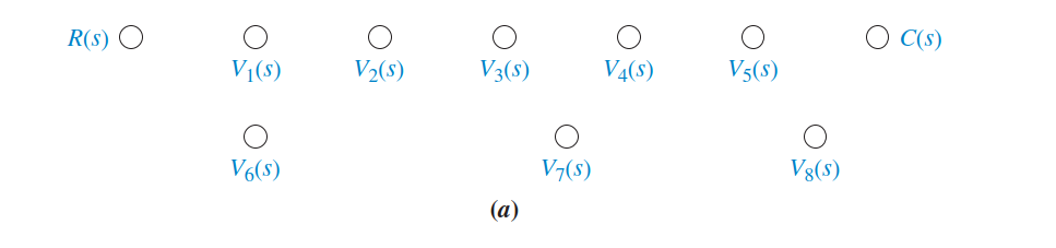
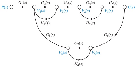
Example 5.7 – Mason’s Rule in Action

Problem: Find \(C(s)/R(s)\) for the signal-flow graph in Figure 5.21.

FIGURE 5.21 – Signal-flow graph for Example 5.7.

Example 5.7 – Step 1: Forward Path

There is one forward path:

• From input \(R(s)\) to output \(C(s)\).

Forward-path gain:

\[ T_1 = G_1(s) G_2(s) G_3(s) G_4(s) G_5(s) \]

Example 5.7 – Step 2: Identify Loop Gains

From the graph, four loops:

1. \[ L_1 = G_2(s) H_1(s) \]

2. \[ L_2 = G_4(s) H_2(s) \]

3. \[ L_3 = G_7(s) H_4(s) \]

4. Large loop through many branches: \[ L_4 = G_2(s)G_3(s)G_4(s)G_5(s)G_6(s)G_7(s)G_8(s) \]

Example 5.7 – Step 3: Nontouching Loops

Check which loops do not share nodes:

• Loop 1 (through \(G_2,H_1\)) does not touch loop 2 (through \(G_4,H_2\)).
• Loop 1 does not touch loop 3 (through \(G_7,H_4\)).
• Loop 2 does not touch loop 3.
• All of 1,2,3 touch loop 4.

Thus, nontouching loop products taken two at a time:

1. \[ L_1 L_2 = G_2H_1G_4H_2 \]

2. \[ L_1 L_3 = G_2H_1G_7H_4 \]

3. \[ L_2 L_3 = G_4H_2G_7H_4 \]

And one triple of nontouching loops:

• Loops 1, 2, and 3: \[ L_1 L_2 L_3 = G_2H_1G_4H_2G_7H_4 \]

No higher-order combinations.

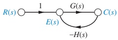
Example 5.7 – Step 4: Compute Δ and Δ₁

Overall \(\Delta\):

\[ \begin{aligned} \Delta = & \;1 - \big[ L_1 + L_2 + L_3 + L_4 \big] \\ & + \big[ L_1L_2 + L_1L_3 + L_2L_3 \big] \\ & - \big[ L_1L_2L_3 \big] \end{aligned} \]

Explicitly:

\[ \begin{aligned} \Delta = & \;1 - \big[ G_2H_1 + G_4H_2 + G_7H_4 \\ & \quad + G_2G_3G_4G_5G_6G_7G_8 \big] \\ & + \big[ G_2H_1G_4H_2 + G_2H_1G_7H_4 + G_4H_2G_7H_4 \big] \\ & - \big[ G_2H_1G_4H_2G_7H_4 \big] \end{aligned} \]

Next, \(\Delta_1\) for the only forward path.

• Remove from \(\Delta\) any loops that touch the forward path nodes.
• From the figure, only loop 3 (with \(G_7H_4\)) does not touch the forward path.

So:

\[ \Delta_1 = 1 - G_7(s)H_4(s) \]

Example 5.7 – Step 5: Final Transfer Function

Apply Mason’s formula:

\[ G(s) = \frac{C(s)}{R(s)} = \frac{T_1 \Delta_1}{\Delta} = \frac{[G_1G_2G_3G_4G_5]\,[1 - G_7H_4]}{\Delta} \]

Highlight that because there is only one forward path, the numerator is just a single term.

In problems with multiple forward paths, we’d have a sum: \(G(s) = (T_1\Delta_1 + T_2\Delta_2 + \dots)/\Delta\).

Encourage students to compare this result with what they’d obtain via block-diagram reduction (for a simpler graph) to see that Mason’s Rule is equivalent but often more systematic.

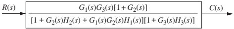
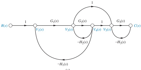
Skill-Assessment Exercise 5.4 – Mason vs. Block Reduction

Problem: Use Mason’s Rule to find the transfer function of the signal-flow graph of Figure 5.19(c).

• This is the same system as Example 5.2, reduced by block diagram algebra.

Answer:

\[ T(s) = \frac{G_{1}(s)G_{3}(s)\big[1 + G_{2}(s)\big]}% {\big[1 + G_{2}(s)H_{2}(s) + G_{1}(s)G_{2}(s)H_{1}(s)\big]\big[1 + G_{3}(s)H_{3}(s)\big]} \]

Note

This demonstrates that:

• Block diagram reduction and Mason’s Rule are equivalent ways to get the same transfer function.
• You can pick whichever is more convenient for a given problem.

In class, you might not derive this fully step-by-step, but you can:

• Show loop and forward-path identification quickly.
• Emphasize that the exact same expression appears whether you use block algebra or Mason’s Rule.

Encourage students to do this derivation on their own for mastery.

Summary / Key Points

• Block diagrams model interconnections of subsystems via blocks, summing junctions, and pickoffs.
• Three key interconnection types:
  • Cascade: multiply transfer functions (if no loading).
  • Parallel: sum transfer functions.
  • Feedback: \(G_{\text{CL}}(s) = \dfrac{G}{1 \pm GH}\).
• Block moves (across summing junctions and pickoffs) are essential to:
  • Expose familiar forms.
  • Systematically reduce complex diagrams.
• Feedback systems often reduce to second-order forms; then:
  • Step response specs (%OS, \(T_s\), \(T_p\), etc.) are set by \(\zeta, \omega_n\).
  • We can design gain \(K\) to meet transient performance requirements.

• Signal-flow graphs:
  • Nodes = signals, branches = transfer functions.
  • Make summing implicit, fit naturally with state-space.
• Mason’s Rule:
  • Provides \(C/R\) in one formula from a signal-flow graph.
  • Requires careful identification of loops and nontouching loops.
• Both block diagram reduction and Mason’s Rule ultimately yield the same transfer function.

Wrap up by connecting back to the chapter learning outcomes:

• We now know how to go from many blocks to one transfer function, both in block-diagram and signal-flow form.
• Next steps (not fully covered today) include mapping to state-space and manipulating similar systems via transformations.

Summary of Key Formulas

Cascade

• For cascade of independent subsystems (no loading):

  \[ G_e(s) = G_n(s) G_{n-1}(s)\dots G_2(s)G_1(s) \]

Parallel

• For parallel subsystems with same input and algebraically summed outputs:

  \[ G_e(s) = \pm G_1(s) \pm G_2(s) \pm \dots \pm G_n(s) \]

Feedback

• Closed-loop transfer function (general feedback):

  \[ G_e(s) = \frac{G(s)}{1 \pm G(s)H(s)} \]

  • Use \(+\) in denominator for negative feedback.

Second-Order Standard Form

• Transfer function:

  \[ T(s) = \frac{\omega_n^{2}}{s^{2} + 2\zeta\omega_n s + \omega_n^{2}} \]

• Relationships:

  • \(\omega_n = \sqrt{\text{constant term}}\).
  • \(2\zeta\omega_n = \text{coefficient of } s\).

• Key transient formulas (for underdamped, \(0<\zeta<1\)):

  • Percent overshoot: \[ \%OS = e^{-\zeta\pi / \sqrt{1-\zeta^{2}}} \times 100 \]

  • Peak time: \[ T_p = \frac{\pi}{\omega_n\sqrt{1-\zeta^{2}}} \]

  • Settling time (2% criterion): \[ T_s = \frac{4}{\zeta\omega_n} \]

Mason’s Rule

• Overall transfer function:

  \[ G(s) = \frac{C(s)}{R(s)} = \frac{\displaystyle\sum_{k} T_k \Delta_k}{\Delta} \]

  Where:

  • \(T_k\) = k-th forward-path gain.

  • \(\Delta = 1 - \sum L_i + \sum L_iL_j - \sum L_iL_jL_k + \dots\)

    • \(L_i\) = individual loop gains.
    • Terms are products of nontouching loop gains with alternating signs.

  • \(\Delta_k = \Delta\) with all loops touching the k-th forward path removed from the expression.

Advise students to keep this “formula page” handy while working homework and labs, especially for Mason’s Rule and the second-order transient formulas.

Suggest a short exercise: take a simple feedback block diagram, write its signal-flow graph, and apply Mason’s Rule to confirm the familiar \(G/(1+GH)\) result.

Interactive Deck

Live Practice: Cascade of Subsystems (No Loading)

Modify the transfer functions and see how the equivalent cascade behaves.

Ask students to: - Change G1, G2, G3 and predict what G_eq will be before running. - Connect this to the formula ( G_e(s) = G_3(s)G_2(s)G_1(s) ) when no loading is present.

Discuss how, in a full transfer-function setting, each ( G_i(s) ) would be a rational function in ( s ), not just a scalar.

Live Practice: Parallel Combination

Experiment with a parallel combination of two subsystems and see their algebraic sum.

Connect to the formula \(G_e(s) = \pm G_1(s) \pm G_2(s) \dots\).

Ask: - What happens if G1 and G2 nearly cancel? - How might this appear in a physical system (e.g., two sensors with opposite polarity)?

Interactive: Closed-Loop Gain from G and H

Play with forward-path and feedback gains and see the closed-loop gain.

We use the standard form:

\[ G_{\text{CL}}(s) = \frac{G(s)}{1 + G(s)H(s)} \]

(assuming negative feedback).

Ask students to: - Increase G while keeping H fixed. What happens to G_cl? Does it saturate? - Relate to control concept: large loop gain can make the closed-loop gain approach \(1/H\), improving tracking and reducing sensitivity.

Reactive: Overshoot vs. Damping Ratio ζ

Use the slider to change damping ratio \(\zeta\), and observe the predicted percent overshoot of a standard second-order system.

viewof zeta = Inputs.range([0.05, 1.2], {step: 0.05, label: "Damping ratio ζ"})

Explain to students: - For underdamped second-order systems (\(0<\zeta<1\)), percent overshoot is \(\%OS = e^{-\zeta\pi/\sqrt{1-\zeta^{2}}}\times 100\). - As ζ increases towards 1, %OS decreases to 0.

Encourage them to find approximate ζ for common overshoots:

• ≈0.7 for about 5% overshoot.
• ≈0.59 for 10% overshoot (as in Example 5.4).

Reactive: Second-Order Step Response (ζ, ωₙ Sliders)

Explore how changing \(\zeta\) and \(\omega_n\) changes the step response of a standard second-order closed-loop system:

\[ T(s) = \frac{\omega_n^2}{s^2 + 2\zeta\omega_n s + \omega_n^2} \]

viewof zeta2 = Inputs.range([0.1, 1.0], {step: 0.05, label: "Damping ratio ζ"})
viewof wn = Inputs.range([0.5, 10.0], {step: 0.5, label: "Natural frequency ωₙ (rad/s)"})

Guide students through:

• Low ζ ⇒ oscillatory, high overshoot.
• Higher ωₙ ⇒ faster oscillations and faster response.
• ζ ≈ 1 ⇒ sluggish but no overshoot (critically damped/overdamped region).

Have them pick a ζ and ωₙ pair that would satisfy, for example, “<10% overshoot and settling time <2s” and describe what they see in the plot.

Reactive: Design K for 10% Overshoot (Example 5.4)

Here we revisit Example 5.4 interactively.

Recall:

\[ T(s) = \frac{K}{s^{2} + 5s + K} \]

For a 10% overshoot, we want \(\zeta \approx 0.591\). Use the slider to choose K and see the resulting ζ and %OS.

viewof K = Inputs.range([1, 50], {step: 0.5, label: "Gain K"})

Ask students: - Adjust K until percent_overshoot is close to 10%. What K do they find? - Compare to the analytical result \(K \approx 17.9\).

This demonstrates inverse design: choose K to realize a desired overshoot.

Reactive: Mason’s Rule – Simple Two-Loop Example

Consider a simple signal-flow graph with:

• Forward path gain \(T_1 = G_1 G_2\).
• A single feedback loop with loop gain \(L_1 = G_2 H\).

For this simple case, Mason’s rule gives:

\[ \Delta = 1 - L_1, \quad \Delta_1 = 1, \quad G(s) = \frac{T_1 \Delta_1}{\Delta} = \frac{G_1 G_2}{1 - G_2 H} \]

Use sliders to change \(G_1, G_2, H\) and observe the resulting transfer function.

viewof G1 = Inputs.range([0.1, 10], {step: 0.1, label: "G₁"})
viewof G2 = Inputs.range([0.1, 10], {step: 0.1, label: "G₂"})
viewof H  = Inputs.range([0.0, 5], {step: 0.1, label: "H"})

Use this to: - Show that Mason’s formula collapses to a familiar feedback expression in simple cases. - Reinforce the definitions: forward path \(T_1\), loop gain \(L_1\), and \(\Delta = 1 - \text{sum of loops}\) when no nontouching loops exist.

Ask students what happens when Delta gets close to zero (i.e., loop gain approaching unity).

Live Practice: Simple Block Moves as Algebra

Treat moving a gain G across a summing junction like factoring in algebra.

Consider:

\[ C(s) = G\big(R(s) - X(s)\big) \quad \text{vs.} \quad C(s) = GR(s) - GX(s) \]

Invite students to edit G, R, and X to see that the equality always holds.

Then connect to moving a block left or right across a summing junction (Figure 5.7): the operation is just factoring/unfactoring in algebra.