Time Response: Analysis of Control Systems

Control 4

Imron Rosyadi

Learning Objectives

After this session, you will be able to:

• Use poles and zeros of transfer functions to determine the time response of a control system.
• Describe quantitatively the transient response of first-order systems.
• Write the general response of second-order systems from pole locations.
• Compute damping ratio \(\zeta\) and natural frequency \(\omega_n\) from a transfer function.
• Find \(T_s\), \(T_p\), %OS, and \(T_r\) for underdamped second-order systems.
• Relate real-world ECE systems (RC/RL, RLC, mechanical) to first- and second-order models.

This list is a subset of the full chapter outcomes, focusing on transient behavior of 1st and 2nd order systems and how pole locations map to time-domain specs.

We will not yet go deep into approximation of higher-order systems or nonlinearities, but we will mention the idea that “dominant poles” often determine behavior.

Motivation: Why Time Response Matters

• Control systems are designed to make outputs follow desired inputs over time.
• Two key aspects:
  • Steady-state behavior (accuracy).
  • Transient behavior (speed, overshoot, oscillation).
• Time response answers questions like:
  • How fast does a motor reach the commanded speed?
  • Does a robot arm overshoot and oscillate?
  • How “snappy” or “sluggish” is an amplifier or filter?

Tip

Think of flicking a light switch vs. motion of an elevator. Both reach a “final value,” but with very different transient behavior.

Emphasize that in many ECE applications—servo drives, power electronics, communication filters—the transient response is often a design constraint: overshoot limits, settling-time requirements, etc.

Students should see time response as something they can specify (requirements) and later meet via controller design.

System Representations: Frequency vs Time

Recall from earlier chapters:

• Transfer functions in the \(s\)-domain (Laplace):
  • Derived from differential equations.
  • Convenient for algebraic manipulation and block diagrams.
• State-space in the time domain:
  • \(\dot{x} = Ax + Bu\)
  • \(y = Cx + Du\)

In this chapter, we:

• Start with a mathematical model (usually a transfer function).
• Use poles and zeros to predict time response.

Remind students they’ve already seen: - How to derive transfer functions from circuits or mechanical systems (Chapter 2). - How to represent systems in state-space (Chapter 3).

Now we’ll exploit these models to understand transient behavior without solving differential equations from scratch each time.

Forced vs Natural Response

Any linear time-invariant (LTI) system output can be decomposed as:

\[ y(t) = y_f(t) + y_n(t) \]

• Forced response \(y_f(t)\):
  • Caused directly by the input.
  • Also called particular solution.
• Natural response \(y_n(t)\):
  • System’s own modes; how it behaves when “left alone.”
  • Decays (or not) based on system poles.

Note

Key idea:

• Input poles \(\Rightarrow\) shape of the forced response.
• System poles \(\Rightarrow\) shape of the natural response.

Stress that “forced” and “natural” correspond to solutions of the non-homogeneous and homogeneous differential equations, respectively.

In practice: - Forced response tells us what type of steady-state we get (step, ramp, sinusoid, etc.). - Natural response tells us about transients: exponentials, oscillations, decay rate.

Poles and Zeros – Definitions

Transfer function: \[ G(s) = \frac{N(s)}{D(s)} \]

• Poles: values of \(s\) where \(G(s)\) becomes infinite.
  • Roots of \(D(s) = 0\).
  • In control we also treat canceled denominator roots as “poles” because they still reflect system dynamics.
• Zeros: values of \(s\) where \(G(s)\) becomes zero.
  • Roots of \(N(s) = 0\).
  • Likewise, canceled numerator roots are still called “zeros” in control.

Important

Even if a pole-zero pair cancels algebraically, the physical mode may still exist. We keep track of them conceptually for design and robustness.

Clarify the subtlety: strictly speaking, only non-canceled denominator roots are mathematical poles. But in control design we often talk about “hidden” or “canceled” poles/zeros because they can reappear with parameter changes or nonlinearities.

Make sure students can define poles and zeros clearly and distinguish numerator vs denominator roles.

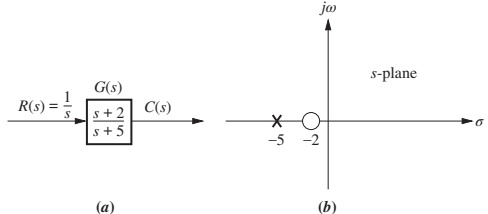
First Example: Simple Pole–Zero System

Given the transfer function (from Fig. 4.1a):

\[ G(s) = \frac{s+2}{s+5} \]

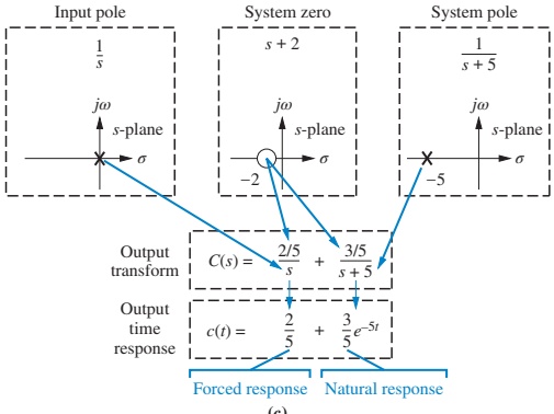
With a unit step input \(R(s) = \frac{1}{s}\),

\[ C(s) = G(s)R(s) = \frac{s+2}{s(s+5)} = \frac{\frac{2}{5}}{s} + \frac{\frac{3}{5}}{s+5} \]

Inverse Laplace transform:

\[ c(t) = \frac{2}{5} + \frac{3}{5} e^{-5t} \]

• Forced response: \(\frac{2}{5}\) (constant step).
• Natural response: \(\frac{3}{5} e^{-5t}\).

Walk through: - The pole at the origin in \(R(s)\) (step input) generated a constant forced component. - The pole at \(s=-5\) in \(G(s)\) generated the \(e^{-5t}\) natural response. - The zero at \(s=-2\) contributed to the coefficients (2/5 and 3/5) but not the basic functional forms.

Highlight that we didn’t need to do heavy algebra to guess the form: - One input pole at 0 → constant term. - One real system pole at -5 → single exponential.

Visualizing Poles and Zeros in the \(s\)-Plane

• Real-axis pole at \(s=-5\).
• Real-axis zero at \(s=-2\).
• Input pole at \(s=0\) (from \(1/s\)).

System and pole-zero plot (Fig. 4.1a,b)

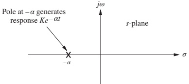
• Real-axis pole \(\Rightarrow\) response term of form \(e^{-\alpha t}\).
• Pole at \(-5\) \(\Rightarrow e^{-5t}\) term.
• The farther left the pole (more negative real part), the faster the exponential decays.

Evolution of response components (Fig. 4.1c)

Ask students: - What happens if the pole is at \(-1\) instead of \(-5\)? → Slower decay (\(e^{-t}\)).

Emphasize: x’s for poles, o’s for zeros. This visual becomes extremely important later for root locus, Bode design, etc.

Takeaways from the Example

From \(C(s) = \frac{s+2}{s(s+5)}\) → \(c(t) = \frac{2}{5} + \frac{3}{5}e^{-5t}\):

1. A pole of the input (at \(s=0\)) generated the forced response (step).
2. A pole of the transfer function (at \(s=-5\)) generated the natural response \(e^{-5t}\).
3. A real-axis pole at \(s=-\alpha\) always generates a term \(e^{-\alpha t}\).
   • More negative \(\alpha\) → faster decay.
4. Zeros and poles together determine the amplitudes of these components (the coefficients 2/5 and 3/5).

Effect of a real-axis pole on transient response (Fig. 4.2)

Stress point (3): this is the first bridge between the s-plane and time response speed. Students should start seeing the left half-plane as a “fast-decay zone” and the right half-plane as unstable.

Link to real systems: RC discharge, current decay in RL circuits, etc., all have real poles.

Example: Response Form by Inspection (Real Poles)

Given (Example 4.1):

\[ R(s) = \frac{1}{s}, \quad G(s) = \frac{s+3}{(s+2)(s+4)(s+5)} \]

By inspection,

\[ C(s) = \frac{K_1}{s} + \frac{K_2}{s+2} + \frac{K_3}{s+4} + \frac{K_4}{s+5} \]

Inverse Laplace:

\[ c(t) = K_1 + K_2 e^{-2t} + K_3 e^{-4t} + K_4 e^{-5t} \]

• \(K_1\) → forced response (step).
• exponentials → natural response.

System with multiple real poles (Fig. 4.3)

Tip

Pattern: each real pole at \(s = -a_i\) adds a term \(e^{-a_i t}\) to the natural response.

Key teaching point: students do not need to compute \(K_i\) to describe the structure of \(c(t)\): - One constant term from input pole at 0. - One exponential per real pole of \(G(s)\).

This “by inspection” capability becomes extremely valuable when reasoning about higher-order systems.

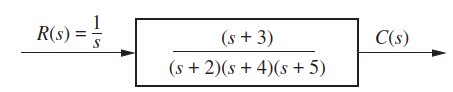
Skill Check – Real Poles

Given: \[ G(s)=\frac{10(s+4)(s+6)}{(s+1)(s+7)(s+8)(s+10)},\quad R(s)=\frac{1}{s} \]

Question: Write the general form of the step response \(c(t)\) by inspection.

Answer:

\[ c(t)\equiv A + B e^{-t} + C e^{-7t} + D e^{-8t} + E e^{-10t} \]

Discuss: - One input pole at \(0\) → constant \(A\). - Four real system poles → four distinct exponentials. - Zeros only affect the coefficients, not the time-function forms.

Encourage students to quickly map: “\(n\) real poles → sum of \(n\) exponentials.”

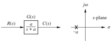
First-Order Systems (No Zeros)

Consider a first-order system (Fig. 4.4a):

\[ G(s) = \frac{a}{s + a},\quad a > 0 \]

With unit step input \(R(s) = \frac{1}{s}\):

\[ C(s)=\frac{a}{s(s+a)} \Rightarrow c(t) = 1 - e^{-at} \]

• Forced response: \(1\) (steady-state).
• Natural response: \(-e^{-at}\) from pole at \(s=-a\) (Fig. 4.4b).

First-order system and pole (Fig. 4.4)

Use a simple RC circuit as analogy: - Input: step voltage source. - Output: capacitor voltage. Transfer function has a single real pole, giving exponential charging.

Emphasize that \(a\) completely characterizes the transient shape here.

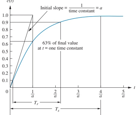
Time Constant of a First-Order System

From \(c(t) = 1 - e^{-at}\):

At \(t = 1/a\):

\[ e^{-at}\big|_{t=1/a} = e^{-1} \approx 0.37 \]

So

\[ c(1/a) = 1 - 0.37 = 0.63 \]

Time constant:

• \(\tau = \dfrac{1}{a}\)
• Time for the step response to reach 63% of its final value.
• Also: time for the exponential \(e^{-at}\) to decay to 37% of its initial value.

First-order step response and time constant (Fig. 4.5)

Note

Pole at \(s=-a\) ↔︎ time constant \(\tau = 1/a\). Farther left pole → smaller \(\tau\) → faster response.

Connect to practical ECE examples: - RC low-pass filter time constant \(RC\). - In op-amp circuits, first-order responses are common when one pole dominates.

Make sure students can translate between time constant and pole location.

First-Order: Rise Time and Settling Time

For \(c(t) = 1 - e^{-at}\):

1. Rise time \(T_r\)

   • Time for \(c(t)\) to go from 10% to 90% of final value:
   • Solve \(1 - e^{-at} = 0.1\) and 0.9, subtract:

   \[ T_r = \frac{2.2}{a} \]

2. Settling time \(T_s\) (2% criterion)

   • Time to reach and stay within 2% of final value.
   • Solve \(1 - e^{-at} = 0.98\):

   \[ T_s = \frac{4}{a} \]

Tip

For a first-order system with pole at \(s=-a\):

• \(\tau = 1/a\)
• \(T_r \approx 2.2\tau\)
• \(T_s \approx 4\tau\)

Point out that these definitions (10–90% rise time, ±2% settling time) are conventional but widely used.

Connect to design: - If you want \(T_s < 0.1\) s, you need \(a > 40\) rad/s.

Identifying a First-Order Transfer Function from Test Data

Real-world scenario:

• You can step the input and measure the output, but do not know internal details.
• If the response looks like a first-order curve (no overshoot, single exponential), you can estimate \(G(s)\) from the step response.

Measured step response (Fig. 4.6)

Procedure:

1. Measure final value \(c_{\infty}\) → equals \(K/a\) for \(G(s) = \dfrac{K}{s+a}\).
2. Measure time constant \(\tau = 1/a\):
   • Time at which \(c(t) \approx 0.63\,c_{\infty}\).
3. Compute \(a = 1/\tau\), then \(K = a\,c_{\infty}\).

In Fig. 4.6:

• \(c_{\infty} \approx 0.72\).
• \(0.63 c_{\infty} \approx 0.45\) at \(t \approx 0.13\) s → \(a \approx 7.7\).
• \(K/a = 0.72 \Rightarrow K \approx 5.54\).
• So \(G(s) \approx \dfrac{5.54}{s+7.7}\).

Highlight that the actual system used \(G(s) = \frac{5}{s+7}\)—our experimental identification is close.

This technique is foundational for system identification and model-based design.

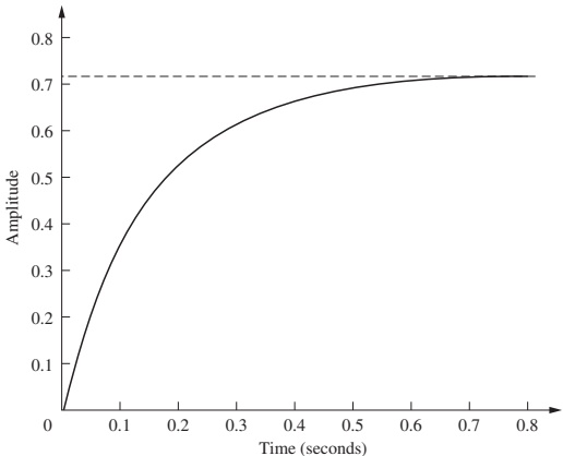
Skill Check – First-Order Specs

Given: \(G(s) = \dfrac{50}{s+50}\)

• Pole at \(s = -50\) → \(a = 50\)
• Time constant: \(\tau = 1/a = 0.02\) s
• Settling time: \(T_s = 4/a = 0.08\) s
• Rise time: \(T_r = 2.2/a \approx 0.044\) s

Answer: \(T_c = 0.02\,\)s, \(T_s = 0.08\,\)s, \(T_r = 0.044\,\)s.

Clarify notation: here \(T_c\) is being used for time constant; earlier we used \(\tau\).

Ask students: - If we double the pole magnitude to 100, how do the times change? → All times halve.

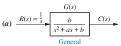
Second-Order Systems – Richer Dynamics

General second-order transfer function (no zeros):

\[ G(s) = \frac{b}{s^{2} + a s + b} \]

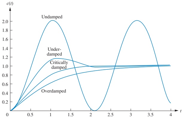
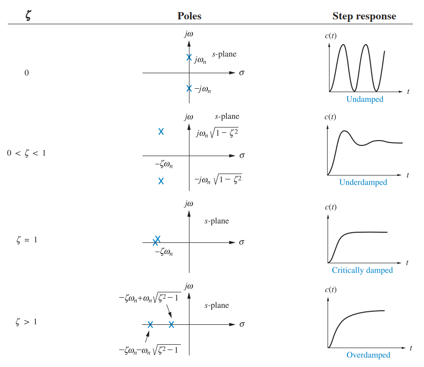
Depending on \(a\) and \(b\), the poles may be:

• Two distinct real poles → overdamped.
• Complex conjugate with negative real part → underdamped.
• Repeated real pole → critically damped.
• Purely imaginary → undamped oscillation.

Second-order cases: pole-zero plots and step responses (Fig. 4.7a–e)

Use Fig. 4.7 set to visually walk through each case: - Overdamped: slow, no overshoot, combination of exponentials. - Underdamped: oscillatory with decaying amplitude. - Undamped: pure oscillation, never settles. - Critically damped: fastest non-overshooting response.

Connect each to typical ECE systems: servo motors, RLC circuits, etc.

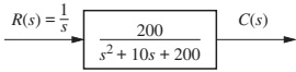
Overdamped Second-Order Response

Example (Fig. 4.7b):

\[ C(s)=\frac{9}{s(s^{2}+9s+9)} =\frac{9}{s(s+7.854)(s+1.146)} \]

• Poles at \(0\), \(-7.854\), \(-1.146\).
• Input pole at 0 → constant forced response.
• Two real system poles → two exponentials in natural response.

Form:

\[ c(t) = K_1 + K_2 e^{-7.854 t} + K_3 e^{-1.146 t} \]

This is an overdamped response: - No oscillation. - Response is sluggish compared to critically damped.

Explain that overdamping often occurs with very high damping (e.g., extremely viscous mechanical systems, heavy smoothing filters).

We can still read off the form directly from the poles, even before computing coefficients.

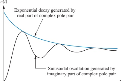
Underdamped Second-Order Response

Example (Fig. 4.7c):

\[ C(s) = \frac{9}{s(s^{2}+2s+9)} \]

System poles at:

\[ s = -1 \pm j\sqrt{8} \]

• Real part \(-1\) → exponential decay rate.
• Imag part \(\sqrt{8}\) → oscillation frequency.

Components of underdamped response (Fig. 4.8)

Form:

\[ c(t) = K_1 + A e^{-t} \cos(\sqrt{8}\,t - \phi) \]

Note

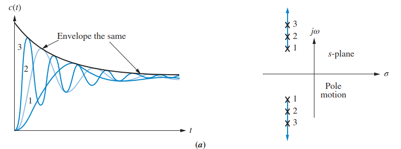
Complex poles \(s = -\sigma_d \pm j\omega_d\) → Natural response \(e^{-\sigma_d t}\cos(\omega_d t - \phi)\).

Explain “damped sinusoid”: - Envelope decays with time constant \(1/\sigma_d\). - Carrier oscillates with radian frequency \(\omega_d\).

Link to RLC circuits: voltage/current ringing after a step.

Example: Form of an Underdamped Response (By Inspection)

Given (Example 4.2, Fig. 4.9):

System with complex poles (Fig. 4.9)

• Transfer function has poles at \(s = -5 \pm j13.23\).
  • Real part \(\sigma_d = 5\) → decay rate \(e^{-5t}\).
  • Imag part \(\omega_d = 13.23\) → oscillation frequency.

Form of step response:

\[ c(t) = K_1 + e^{-5t}\left(K_2\cos 13.23 t + K_3\sin 13.23 t\right) \]

or

\[ c(t) = K_1 + K_4 e^{-5t}\cos(13.23 t - \phi) \]

Highlight the structure: - Constant + damped sinusoid. - You can always combine \(K_2\cos + K_3\sin\) into a shifted cosine with amplitude \(K_4\) and phase \(\phi\).

Students should practice going from complex poles to this form without solving partial fractions.

Undamped and Critically Damped Cases

1. Undamped (Fig. 4.7d):

   \[ C(s) = \frac{9}{s(s^2+9)} \]

   • Poles at \(0\), \(\pm j3\).
   • Form: \(c(t) = K_1 + K_4 \cos(3t - \phi)\).
   • No decay; pure oscillation.

2. Critically damped (Fig. 4.7e):

   \[ C(s) = \frac{9}{s(s^2+6s+9)} = \frac{9}{s(s+3)^2} \]

   • Poles at \(0\), \(-3\) (double).
   • Form: \(c(t) = K_1 + K_2 e^{-3t} + K_3 t e^{-3t}\).
   • Fastest response possible without overshoot.

Second-order step responses for different damping cases (Fig. 4.10)

Make clear: - Multiple real poles (critical damping) lead to terms like \(t e^{-\sigma t}\). - Undamped case (pure imaginary poles) is often an idealization; in reality, there is almost always some damping.

Use Fig. 4.10 to compare all four damping cases on the same axes.

Summary: Natural Responses for Second-Order Systems

1. Overdamped (\(\zeta > 1\)):
   • Poles: \(-\sigma_1\), \(-\sigma_2\) real, distinct.
   • Natural response: \[ c_n(t) = K_1 e^{-\sigma_1 t} + K_2 e^{-\sigma_2 t} \]
2. Underdamped (\(0 < \zeta < 1\)):
   • Poles: \(-\sigma_d \pm j\omega_d\).
   • Natural response: \[ c_n(t) = A e^{-\sigma_d t}\cos(\omega_d t - \phi) \]

3. Undamped (\(\zeta = 0\)):
   • Poles: \(\pm j\omega_1\).
   • Natural response: \[ c_n(t) = A\cos(\omega_1 t - \phi) \]
4. Critically damped (\(\zeta = 1\)):
   • Poles: repeated real \(-\sigma_1\).
   • Natural response: \[ c_n(t) = K_1 e^{-\sigma_1 t} + K_2 t e^{-\sigma_1 t} \]

At this point, ensure students can classify a given second-order denominator into one of these cases by checking discriminant or computing \(\zeta\).

Soon we’ll formalize \(\zeta\) and \(\omega_n\) and link them to these behaviors.

Skill Check – Classify Second-Order Responses

Given the transfer functions:

1. \(G(s) = \dfrac{400}{s^{2}+12s+400}\)

2. \(G(s) = \dfrac{900}{s^{2}+90s+900}\)

3. \(G(s) = \dfrac{225}{s^{2}+30s+225}\)

4. \(G(s) = \dfrac{625}{s^{2}+625}\)

By inspection, the step responses are:

1. \(c(t)=A+B e^{-6t}\cos(19.08t+\phi)\) (underdamped)

2. \(c(t)=A+B e^{-78.54t}+C e^{-11.46t}\) (overdamped)

3. \(c(t)=A+B e^{-15t}+C t e^{-15t}\) (critically damped)

4. \(c(t)=A+B\cos(25t+\phi)\) (undamped)

Encourage students to:

• Factor or complete the square.
• Recognize complex vs real roots quickly.
• Map roots to the patterns from the summary slide.

This will prepare them for computing \(\zeta\) and \(\omega_n\) next.

General Second-Order System in Standard Form

We rewrite

\[ G(s) = \frac{b}{s^{2} + a s + b} \]

in terms of natural frequency \(\omega_n\) and damping ratio \(\zeta\):

1. Set \(b = \omega_n^2\) → undamped poles at \(\pm j\omega_n\).

2. Use definition of damping ratio:

   \[ \zeta = \frac{\text{decay frequency}}{\text{natural frequency}} = \frac{|\sigma|}{\omega_n} \]

   For underdamped case, poles: \(s = -\frac{a}{2} \pm j\cdots\) → \(|\sigma| = a/2\).

   So

   \[ \zeta = \frac{a/2}{\omega_n} \Rightarrow a = 2\zeta \omega_n \]

Thus the standard form is:

\[ G(s) = \frac{\omega_n^{2}}{s^{2} + 2\zeta\omega_n s + \omega_n^{2}} \]

Emphasize that every second-order system (no zeros) can be rewritten in this standard form.

This form: - Makes \(\omega_n\) and \(\zeta\) explicit. - Lets us use tables/plots that relate these parameters to transient specs.

Example: Find \(\zeta\) and \(\omega_n\) from \(G(s)\)

(Example 4.3)

Given:

\[ G(s) = \frac{36}{s^2 + 4.2s + 36} \]

Compare with

\[ \frac{\omega_n^2}{s^2 + 2\zeta\omega_n s + \omega_n^2} \]

• \(\omega_n^2 = 36\) → \(\omega_n = 6\).
• \(2\zeta\omega_n = 4.2 \Rightarrow 2\zeta(6) = 4.2 \Rightarrow \zeta = 0.35\).

So:

• \(\omega_n = 6\) rad/s.
• \(\zeta = 0.35\) → underdamped.

Have students quickly check: - \(\zeta < 1\) → underdamped, consistent with expectation of oscillatory response.

This pattern (compare numerator to \(\omega_n^2\), denominator to \(s^2 + 2\zeta\omega_n s + \omega_n^2\)) will be used repeatedly.

Poles of the Standard Second-Order System

For

\[ G(s) = \frac{\omega_n^{2}}{s^{2} + 2\zeta\omega_n s + \omega_n^{2}}, \]

the poles are:

\[ s_{1,2} = -\zeta\omega_n \pm \omega_n\sqrt{\zeta^{2} - 1} \]

• If \(0 < \zeta < 1\) → complex conjugate pair (underdamped).
• If \(\zeta = 1\) → repeated real pole (critical).
• If \(\zeta > 1\) → two real distinct poles (overdamped).
• If \(\zeta = 0\) → purely imaginary poles (undamped).

Second-order response as a function of \(\zeta\) (Fig. 4.11)

Show Fig. 4.11 to illustrate how shifting \(\zeta\) sweeps through all damping cases.

Students should memorize: - \(\zeta\) near 0 → highly oscillatory. - \(\zeta\) near 1 → critically damped, no overshoot. - \(\zeta > 1\) → more sluggish than critical.

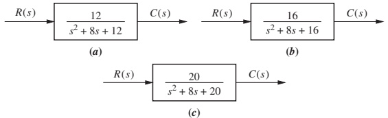
Example: Classifying Response from \(\zeta\)

(Example 4.4, Fig. 4.12)

Given several systems of form:

\[ G(s) = \frac{b}{s^2 + a s + b} \]

We use:

\[ \zeta = \frac{a}{2\sqrt{b}} \]

to compute \(\zeta\) and classify:

• If \(\zeta > 1\) → overdamped.
• If \(\zeta = 1\) → critically damped.
• If \(0 < \zeta < 1\) → underdamped.

For the three systems in Fig. 4.12:

• System (a): \(\zeta = 1.155\) → overdamped.
• System (b): \(\zeta = 1\) → critically damped.
• System (c): \(\zeta = 0.894\) → underdamped.

Systems for Example 4.4

Work through one numerically on the board.

For example, if \(G(s) = \frac{16}{s^2+8s+16}\): - \(a=8\), \(b=16\), so \(\zeta = 8/(2*4) = 1\) → critically damped.

Underdamped Second-Order Step Response

For underdamped \(0 < \zeta < 1\):

\[ G(s) = \frac{\omega_n^{2}}{s^{2} + 2\zeta\omega_n s + \omega_n^{2}} \]

With unit step input \(R(s) = \frac{1}{s}\):

\[ C(s) = \frac{\omega_n^{2}}{s(s^{2} + 2\zeta\omega_n s + \omega_n^{2})} \]

After partial fractions and inverse Laplace (derivation omitted):

\[ \begin{aligned} c(t) &= 1 - e^{-\zeta\omega_n t}\Bigg( \cos\omega_n\sqrt{1-\zeta^{2}}\, t + \frac{\zeta}{\sqrt{1-\zeta^{2}}}\sin\omega_n\sqrt{1-\zeta^{2}}\, t \Bigg) \\ &= 1 - \frac{1}{\sqrt{1-\zeta^{2}}} e^{-\zeta\omega_n t} \cos\big(\omega_n\sqrt{1-\zeta^{2}}\, t - \phi\big) \end{aligned} \]

where

\[ \phi = \tan^{-1}\left(\frac{\zeta}{\sqrt{1 - \zeta^2}}\right) \]

Underdamped responses for different \(\zeta\) (Fig. 4.13)

Clarify:

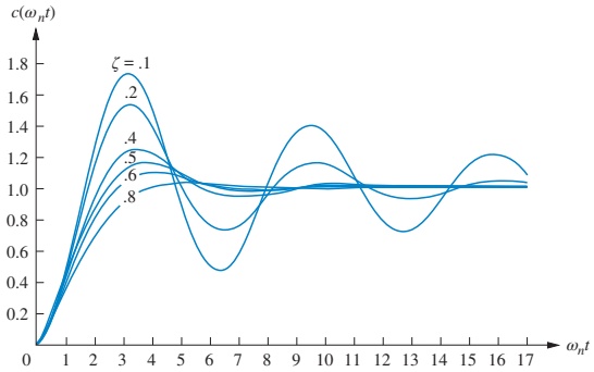
• As \(\zeta\) decreases, oscillations become more prominent and last longer.
• \(\omega_n\) mainly scales the time axis; \(\zeta\) controls the shape.

We will extract \(T_p\), %OS, \(T_s\), and \(T_r\) from this expression.

Under-damped Specs: Definitions

For the underdamped step response (Fig. 4.14):

Underdamped response specs (Fig. 4.14)

Definitions:

1. Rise time \(T_r\) — time to go from 10% to 90% of final value.
2. Peak time \(T_p\) — time to the first (maximum) peak.
3. Percent overshoot %OS — \[ \%OS = \frac{c_{\max} - c_{\text{final}}}{c_{\text{final}}} \times 100\% \]
4. Settling time \(T_s\) — time to enter and stay within \(\pm 2\%\) of final value.

Reinforce that these definitions generalize beyond second-order systems but are exactly computable only for the standard second-order case.

Later, for higher-order systems, we often approximate them as dominated by a pair of complex conjugate poles.

Deriving Peak Time \(T_p\)

For \(c(t)\) given earlier:

• Differentiate \(c(t)\), set \(\dot{c}(t)=0\) to find extrema.
• Using Laplace differentiation property,

\[ \mathcal{L}[\dot{c}(t)] = sC(s) = \frac{\omega_n^2}{s^{2}+2\zeta\omega_ns+\omega_n^{2}} \]

Inverse Laplace gives:

\[ \dot{c}(t) = \frac{\omega_n}{\sqrt{1-\zeta^2}} e^{-\zeta\omega_n t} \sin\left(\omega_n\sqrt{1-\zeta^2}\,t\right) \]

Set \(\dot{c}(t)=0\):

\[ \omega_n\sqrt{1-\zeta^2}\,t = n\pi \Rightarrow t = \frac{n\pi}{\omega_n\sqrt{1-\zeta^2}} \]

First nonzero peak: \(n = 1\) →

\[ T_p = \frac{\pi}{\omega_n\sqrt{1-\zeta^2}} \]

Interpretation: - \(\omega_d = \omega_n\sqrt{1-\zeta^2}\) is the damped natural frequency. - So \(T_p = \pi/\omega_d\).

Students should memorize this formula; it will be heavily used in design problems.

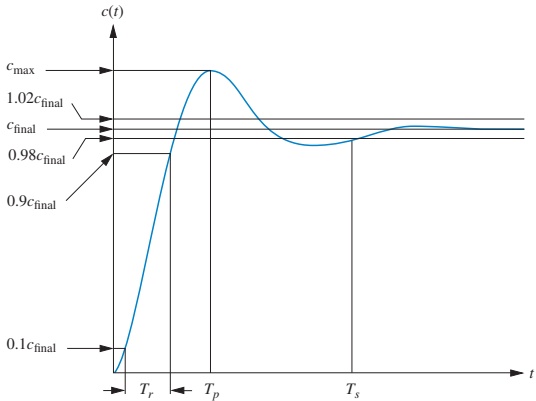
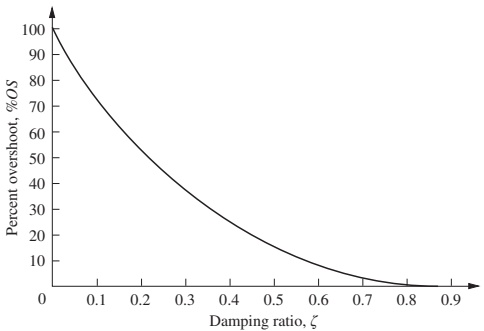
Deriving Percent Overshoot %OS

From the definition:

\[ \%OS = \frac{c_{\max} - c_{\text{final}}}{c_{\text{final}}}\times100 \]

For a unit step, \(c_{\text{final}} = 1\).

Evaluate \(c(t)\) at \(t = T_p\):

\[ c_{\max} = c(T_p) = 1 + e^{-\frac{\zeta\pi}{\sqrt{1-\zeta^2}}} \]

So

\[ \%OS = e^{-\frac{\zeta\pi}{\sqrt{1-\zeta^2}}}\times100 \]

This depends only on \(\zeta\).

Percent overshoot vs damping ratio (Fig. 4.15)

Inverse relationship:

\[ \zeta = \frac{-\ln(\%OS/100)}{\sqrt{\pi^2 + \ln^2(\%OS/100)}} \]

Tip

Design trick: If the specs give you maximum %OS, use this formula to compute \(\zeta\).

Walk through a quick example: - For 20% overshoot: \(\%OS=20\) → \(\zeta\approx 0.456\).

This will be used again in the design example with the mechanical system.

Deriving Settling Time \(T_s\)

We want \(|c(t) - 1| \le 0.02\) for all \(t \ge T_s\).

Approximate envelope of oscillation from \(c(t)\):

\[ \left|\frac{1}{\sqrt{1-\zeta^2}}e^{-\zeta\omega_n t}\right| \le 0.02 \]

Solve

\[ \frac{1}{\sqrt{1-\zeta^2}}e^{-\zeta\omega_n t} = 0.02 \]

\[ T_s = \frac{-\ln(0.02\sqrt{1-\zeta^2})}{\zeta\omega_n} \]

Numerator changes slowly with \(\zeta\); we often approximate:

\[ T_s \approx \frac{4}{\zeta\omega_n} \]

Explain: - Numerator ranges roughly 3.9–4.7 over typical \(\zeta\) values. - Using 4 is a convenient engineering approximation (“4 time constants”).

Reinforce that \(T_s\) is dominated by the real part of the poles: larger \(\zeta\omega_n\) → faster decay.

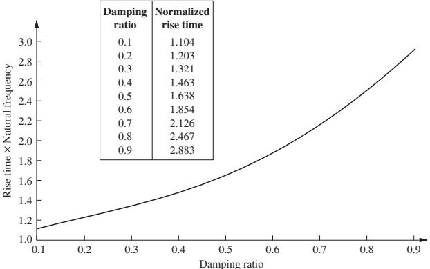
Rise Time \(T_r\) for Underdamped Systems

There is no simple closed-form formula like for \(T_p\) or \(T_s\).

Approach:

• Normalize time by \(\omega_n\) (use variable \(\omega_n t\)).
• For a given \(\zeta\), numerically solve
  • \(c(t) = 0.1\) and \(c(t) = 0.9\),
  • Then \(T_r = t_{0.9} - t_{0.1}\).

Result (computed values) plotted as normalized rise time:

Normalized rise time vs \(\zeta\) (Fig. 4.16)

Given \(\zeta\) and \(\omega_n\):

• Find \(\omega_n T_r\) from the plot/table.
• Then \(T_r = (\omega_n T_r)/\omega_n\).

For design work, you will often: - Use the plot (or a lookup table) for normalized \(T_r\) vs \(\zeta\). - Combine with \(T_p\), \(T_s\), and %OS to choose acceptable \(\zeta\) and \(\omega_n\).

Point out the trend: smaller \(\zeta\) usually means smaller \(T_r\) but more overshoot.

Example: Compute \(T_p\), %OS, \(T_s\), \(T_r\)

(Example 4.5)

Given

\[ G(s) = \frac{100}{s^2 + 15s + 100} \]

1. Put in standard form:

   • \(\omega_n^2 = 100\) → \(\omega_n = 10\).
   • \(2\zeta\omega_n = 15\) → \(\zeta = \frac{15}{2\cdot10} = 0.75\).

2. Use formulas:

   • \(T_p = \dfrac{\pi}{\omega_n\sqrt{1-\zeta^{2}}} = \dfrac{\pi}{10\sqrt{1-0.75^2}} \approx 0.475\,\)s.

   • \(\%OS = e^{-\zeta\pi/\sqrt{1-\zeta^2}}\times100 \approx 2.84\%\).

   • \(T_s \approx \dfrac{4}{\zeta\omega_n} = \dfrac{4}{0.75\cdot10} \approx 0.533\,\)s.

   • From Fig. 4.16, for \(\zeta=0.75\), \(\omega_n T_r \approx 2.3\) → \(T_r = 2.3/10 = 0.23\,\)s.

Key lesson: we obtained all major time-domain specs without ever computing \(c(t)\) explicitly.

Students should recognize this as a powerful shortcut that will be used repeatedly in later chapters (root locus, PID tuning, etc.).

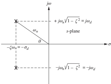
Geometric Interpretation in the \(s\)-Plane

For underdamped poles:

\[ s_{1,2} = -\zeta\omega_n \pm j\omega_n\sqrt{1-\zeta^2} \]

In the \(s\)-plane (Fig. 4.17):

Pole plot for underdamped second-order system (Fig. 4.17)

• Radial distance from origin: \(\omega_n\).
• Angle \(\theta\) from negative real axis: \(\cos\theta = \zeta\).
• Real part magnitude: \(\sigma_d = \zeta\omega_n\).
• Imag part: \(\omega_d = \omega_n\sqrt{1-\zeta^2}\).

Time-domain specs in terms of pole coordinates:

• \(T_p = \dfrac{\pi}{\omega_d}\).
• \(T_s \approx \dfrac{4}{\sigma_d}\).

Note

Lines of: - constant \(\zeta\) → rays from origin (constant angle). - constant \(T_p\) → horizontal lines (constant imaginary part). - constant \(T_s\) → vertical lines (constant real part).

This geometric picture is central for design: - Moving poles left → smaller \(T_s\). - Moving poles up/down → changes oscillation period and \(T_p\). - Moving poles along a ray from origin → keep %OS constant but scale time.

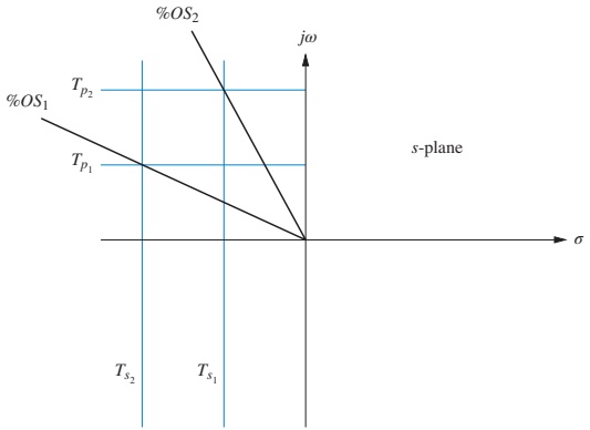
Lines of Constant \(T_p\), \(T_s\), and %OS

Lines of constant \(T_p\), \(T_s\), and %OS (Fig. 4.18)

Interpretation:

• Vertical lines: same real part → same exponential damping → approximate same \(T_s\).
• Horizontal lines: same imaginary part → same oscillation frequency → same \(T_p\).
• Radial lines: same \(\zeta\) → same %OS.

Use this picture to preview control design: - In root locus design, controller gains “slide” poles along trajectories in the \(s\)-plane. - Designers choose a target region in the \(s\)-plane satisfying constraints on overshoot and speed.

Show that as you move outwards along a constant \(\zeta\) ray, the time response looks similar but scaled in time.

How Pole Movement Affects Response

Step responses as poles move (Fig. 4.19a–c)

1. Move poles vertically (constant real part) → Fig. 4.19(a):
   • Same decay envelope (same \(\sigma_d\) → same \(T_s\)).
   • Higher imaginary part → faster oscillation, smaller \(T_p\), higher overshoot.
2. Move poles horizontally (constant imaginary part) → Fig. 4.19(b):
   • Same oscillation frequency, same \(T_p\).
   • Larger real part (farther left) → faster decay, smaller \(T_s\), smaller overshoot.
3. Move radially (constant \(\zeta\)) → Fig. 4.19(c):
   • Same %OS.
   • Larger distance from origin → faster response overall (both \(T_p\) and \(T_s\) smaller).

Encourage students to relate these observations to Eq. (4.44) and (4.45).

This intuition is key for closed-loop design: we will eventually “aim” closed-loop poles into a desired region for acceptable transient response.

Example: Time Specs from Pole Location

(Example 4.6)

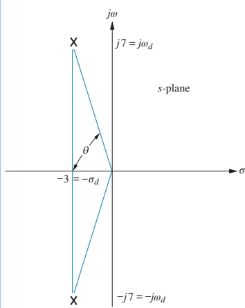
Given poles at (Fig. 4.20):

Pole plot for Example 4.6

• Real part: \(-3\) → \(\sigma_d = 3\).
• Imag part: \(7\) → \(\omega_d = 7\).
• Radial distance: \(\omega_n = \sqrt{3^2 + 7^2} = 7.616\).
• Angle: \(\theta = \tan^{-1}(7/3)\) → \(\zeta = \cos\theta = 0.394\).

Now compute:

• \(T_p = \dfrac{\pi}{\omega_d} = \dfrac{\pi}{7} \approx 0.449\,\)s.

• \(\%OS = e^{-\zeta\pi/\sqrt{1-\zeta^2}}\times100 \approx 26\%\).

• \(T_s \approx \dfrac{4}{\sigma_d} = \dfrac{4}{3} \approx 1.33\,\)s.

We never used the actual transfer function, only the pole locations.

This is often how design specs are enforced: given allowed \(T_s\) and %OS, determine acceptable regions for poles.

Design Example: Mechanical System Specs → Component Values

(Example 4.7)

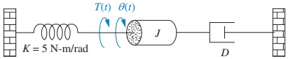
Rotational mechanical system (Fig. 4.21):

Rotational system for Example 4.7

Transfer function:

\[ G(s) = \frac{\Theta(s)}{T(s)} = \frac{1/J}{s^2 + (D/J)s + (K/J)} \]

Put in standard form:

• \(\omega_n^2 = K/J \Rightarrow \omega_n = \sqrt{K/J}\).
• \(2\zeta\omega_n = D/J\).

Specifications:

• %OS = 20% → from Eq. (4.39), \(\zeta \approx 0.456\).

• \(T_s = 2\) s → from \(T_s = 4/(\zeta\omega_n)\):

  \[ 2 = \frac{4}{\zeta\omega_n} \Rightarrow \zeta\omega_n = 2 \]

Thus:

• \(2\zeta\omega_n = 4 = D/J\).

• From \(\zeta = 2\sqrt{J/K}\) (algebra), and \(\zeta = 0.456\),

  \[ 2\sqrt{\frac{J}{K}} = 0.456 \Rightarrow \frac{J}{K} \approx 0.052 \]

Given \(K = 5\,\mathrm{N\cdot m/rad}\):

• \(J = 0.052 K = 0.26\,\mathrm{kg\cdot m^2}\).
• From \(D/J = 4\), \(D = 4J = 1.04\,\mathrm{N\cdot m\cdot s/rad}\).

Important

We translated time-domain specs (overshoot and settling time) into physical design parameters \(J\) and \(D\).

This example closes the loop between:

• Desired behavior (20% overshoot, 2 s settling).
• Abstract parameters (\(\zeta\), \(\omega_n\)).
• Concrete hardware values (\(J\), \(D\), \(K\)).

It anticipates later chapters where we do the same via controller gains instead of just plant parameters.

Skill Check – Complete Spec from \(G(s)\)

(Exercise 4.5)

Given:

\[ G(s) = \frac{361}{s^{2}+16s+361} \]

1. \(\omega_n^{2} = 361 \Rightarrow \omega_n = 19\).
2. \(2\zeta\omega_n = 16 \Rightarrow \zeta = \frac{16}{2\cdot 19} = 0.421\).
3. \(T_s \approx \frac{4}{\zeta\omega_n} = \frac{4}{0.421\cdot19} \approx 0.5\) s.
4. \(T_p = \frac{\pi}{\omega_n\sqrt{1-\zeta^{2}}} \approx 0.182\) s.
5. From Fig. 4.16: \(\omega_n T_r \approx 1.5\) (for \(\zeta\approx 0.42\)) → \(T_r \approx 0.079\) s.
6. \(\%OS = e^{-\zeta\pi/\sqrt{1-\zeta^2}}\times100 \approx 23.3\%\).

Encourage students to check each computation carefully, especially %OS.

This exercise ties together all main formulas and shows the power of the standard second-order form.

Summary / Key Points

• Poles and zeros give a powerful, often qualitative way to predict time response:
  • Input poles → forced response shape.
  • System poles → natural response shape.
  • Zeros and poles determine amplitudes.
• First-order systems:
  • Step response: \(1 - e^{-at}\).
  • Time constant \(\tau = 1/a\) fully characterizes transient speed.
  • \(T_r \approx 2.2\tau\), \(T_s \approx 4\tau\).
• Second-order systems:
  • Standard form: \(\dfrac{\omega_n^2}{s^2+2\zeta\omega_n s+\omega_n^2}\).
  • \(\omega_n\) sets time scale; \(\zeta\) sets damping/shape.
  • Behavior classification: overdamped, critically damped, underdamped, undamped.

• Underdamped second-order step response:
  • \(T_p = \dfrac{\pi}{\omega_n\sqrt{1-\zeta^2}}\).
  • \(\%OS = e^{-\zeta\pi/\sqrt{1-\zeta^2}}\times100\).
  • \(T_s \approx \dfrac{4}{\zeta\omega_n}\).
  • \(T_r\) from normalized curves vs \(\zeta\).
• s-plane geometry:
  • Lines of constant \(\zeta\), \(T_p\), \(T_s\), and %OS provide an intuitive design map.

Encourage students to: - Memorize the standard 2nd-order form and the core formulas (for \(T_p\), %OS, \(T_s\)). - Practice reading pole locations as “coordinates of transient behavior.” - Start thinking about how changing system or controller parameters moves poles in the s-plane.

Formulas Summary – First- & Second-Order Time Response

First-order system

• Transfer function: \[ G(s) = \frac{K}{s+a},\quad a>0 \]

• Unit step response: \[ c(t) = \frac{K}{a}\left(1-e^{-at}\right) \]

• Time constant: \(\tau = 1/a\).

• Rise time (10–90%): \(T_r \approx 2.2/a = 2.2\tau\).

• Settling time (2%): \(T_s \approx 4/a = 4\tau\).

Second-order standard form

• Transfer function: \[ G(s) = \frac{\omega_n^{2}}{s^{2}+2\zeta\omega_n s+\omega_n^{2}} \]

• Poles: \[ s_{1,2} = -\zeta\omega_n \pm j\omega_n\sqrt{1-\zeta^{2}} \]

• Damped natural frequency: \[ \omega_d = \omega_n\sqrt{1-\zeta^{2}} \]

Underdamped second-order (unit step)

• Response: \[ c(t) = 1 - \frac{1}{\sqrt{1-\zeta^{2}}}e^{-\zeta\omega_n t} \cos(\omega_n\sqrt{1-\zeta^{2}}\, t - \phi) \]

• Peak time: \[ T_p = \frac{\pi}{\omega_n\sqrt{1-\zeta^{2}}} = \frac{\pi}{\omega_d} \]

• Percent overshoot: \[ \%OS = e^{-\frac{\zeta\pi}{\sqrt{1-\zeta^{2}}}}\times100 \]

• Inverse relation: \[ \zeta = \frac{-\ln(\%OS/100)}{\sqrt{\pi^{2}+\ln^{2}(\%OS/100)}} \]

• Settling time (2%): \[ T_s \approx \frac{4}{\zeta\omega_n} \]

• Rise time: \[ \omega_n T_r \text{ from lookup vs. } \zeta,\quad T_r = \frac{\omega_n T_r}{\omega_n} \]

This slide can serve as a quick reference sheet for homework and exams.

Suggest to students: - Keep this summary handy when solving problems. - Practice deriving selected formulas once to understand them, then memorize for speed.

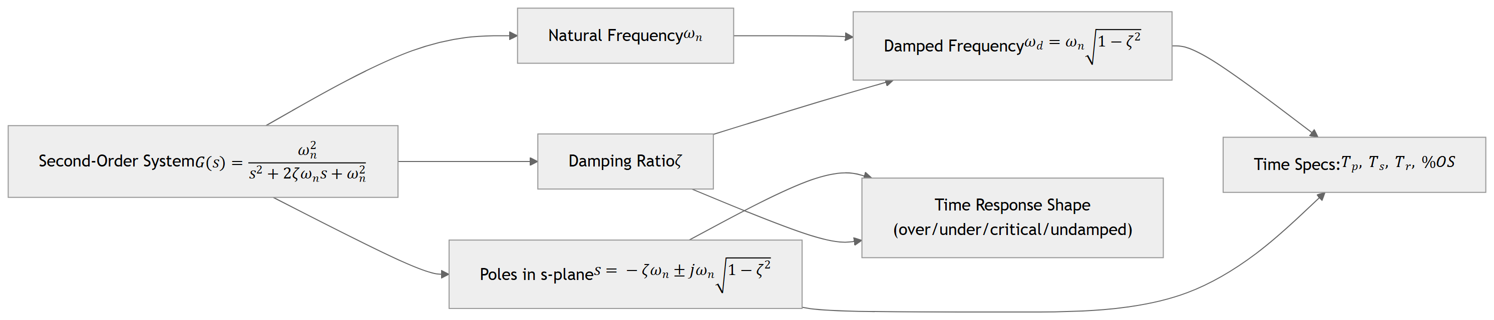
Optional Concept Map (Mermaid Diagram)

Use this concept map to reinforce how: - \(G(s)\) determines poles and \((\zeta,\omega_n)\). - Poles determine geometry in \(s\)-plane. - Geometry and \((\zeta,\omega_n)\) determine time-domain specs and the qualitative shape of the response.

Time Response – Interactive Deck

Getting Started: Live Python in the Browser

You can run Python code directly in this slide using Pyodide.

Try modifying the parameters and re-running.

Have students: - Change a to several values (e.g., 1, 2, 5, 10, 50). - Observe how the time constant and settling time scale.

This introduces them to the idea that pole location determines response speed.

Interactive: First-Order Step Response Shape

Explore how the first-order step response

\[ c(t) = 1 - e^{-a t} \]

changes as the pole location \(s=-a\) moves.

Ask: - Increase a — what happens to the response speed? - How does this relate to the pole moving farther left on the real axis?

Students should see that larger a → faster rise and settling.

Reactive Controls: First-Order System Explorer

Use the slider to change the pole location \(s=-a\) and see how the step response changes.

viewof a_fo = Inputs.range(
  [0.5, 20],
  {step: 0.5, label: "First-order pole magnitude a (pole at s = -a)"}
)

Guide questions: - Move the slider to small a (near 0.5). What happens to \(T_s\)? - Move to large a (near 20). How does the response change?

Students should connect: - \(T_s \approx 4/a\). - The graphical interpretation: how long until the curve stays close to 1.

Interactive: Second-Order Parameters from Coefficients

Given

\[ G(s) = \frac{b}{s^2 + a s + b} \]

we have

\[ \omega_n = \sqrt{b}, \quad \zeta = \frac{a}{2\sqrt{b}} \]

Try changing \(a\) and \(b\) and see how \(\zeta\) and \(\omega_n\) change.

Have students: - Try a combination that yields \(\zeta < 1\) (e.g., \(a=4.2\), \(b=36\)). - Try a large \(a\) to get \(\zeta > 1\). - Observe how the classification changes.

This builds intuition on how numerator/denominator coefficients relate to damping.

Reactive: Second-Order \((\zeta, \omega_n)\) → Time Specs

Use sliders to pick \(\zeta\) and \(\omega_n\), then see \(T_p\), \(T_s\), and %OS.

viewof zeta = Inputs.range(
  [0.0, 1.0],
  {step: 0.02, label: "Damping ratio ζ (0 ≤ ζ ≤ 1)"}
)
viewof omega_n = Inputs.range(
  [1, 30],
  {step: 1, label: "Natural frequency ω_n (rad/s)"}
)

Ask: - For fixed \(\zeta\), increase \(\omega_n\). What happens to \(T_p\) and \(T_s\)? - For fixed \(\omega_n\), change \(\zeta\). How do \(T_p\), \(T_s\), and %OS change?

They should see that: - Larger \(\omega_n\) scales time faster (shorter \(T_p\), \(T_s\)). - Larger \(\zeta\) reduces overshoot and also changes \(T_p\), \(T_s\).

Reactive Plot: Underdamped Second-Order Step Response

Now visualize the full step response for your chosen \((\zeta, \omega_n)\).

Have students: - Choose \(\zeta\) near 0.2: see large overshoot and long ringing. - Choose \(\zeta\) near 0.7–0.8: small overshoot, fast settling. - Compare with earlier formulas for %OS and \(T_s\).

This integrates formulas with direct visual intuition.

Reactive: From Poles in the \(s\)-Plane to Time Specs

Use sliders to set the real and imaginary parts of a complex pole pair \(s = -\sigma_d \pm j\omega_d\) (under-damped case only, \(\sigma_d>0\), \(\omega_d>0\)).

viewof sigma_d = Inputs.range(
  [0.5, 10],
  {step: 0.5, label: "Real part σ_d (>0) (damping rate)"}
)
viewof omega_d = Inputs.range(
  [0.5, 20],
  {step: 0.5, label: "Imag part ω_d (>0) (oscillation frequency)"}
)

Questions to explore: - For fixed \(\sigma_d\), increase \(\omega_d\): how does \(T_p\) change? - For fixed \(\omega_d\), increase \(\sigma_d\): how does \(T_s\) and %OS change?

Connect back to the “lines of constant \(T_p\), \(T_s\), and %OS” slide in the main deck.

Reactive Plot: Pole Location and Step Response Together

This block simultaneously shows:

• Pole positions in the \(s\)-plane.
• Corresponding underdamped step response.

Encourage: - Move poles farther left (increase σ_d) → watch response settle faster. - Move poles up/down (change ωd) → frequency of oscillation and \(T_p\) change, while envelope slope (\(σ_d\)) stays same.

This is a direct visual of “move poles, change time response.”

Design Sandbox: Meet a %OS and \(T_s\) Spec

Suppose we want an underdamped second-order system with:

• Max %OS requirement: \(\leq\) given spec.
• Settling time \(T_s\) requirement: \(\leq\) given spec.

We’ll: 1. Choose a %OS spec, compute \(\zeta\). 2. Choose a \(T_s\) spec, compute \(\omega_n\). 3. Show the resulting step response.

viewof OS_spec = Inputs.range(
  [1, 40],
  {step: 1, label: "Desired maximum %OS (1–40%)"}
)
viewof Ts_spec = Inputs.range(
  [0.1, 5],
  {step: 0.1, label: "Desired maximum settling time Ts (s)"}
)

Guide students: - Set %OS_spec to 5% and Ts_spec to 1 s; observe ζ and ω_n. - Then relax Ts_spec (e.g., 3 s) and see how ω_n changes. - Experiment with more aggressive specs and see how ζ, ω_n, and the response behave.

This mimics a basic design workflow: time-domain specs → \((\zeta, \omega_n)\) → system behavior.

Wrap-Up Interactive Reflections

Use the editors and reactive controls to answer:

1. How does moving real poles left or right impact:
   • First-order response speed?
   • Second-order \(T_s\) and \(T_p\)?
2. How does changing damping ratio \(\zeta\) at fixed \(\omega_n\) affect:
   • Percent overshoot?
   • Number of oscillations before settling?
3. For a given performance requirement (e.g., \(T_s\) and %OS), can you:
   • Compute suitable \(\zeta\) and \(\omega_n\)?
   • Sketch approximate pole locations in the \(s\)-plane?

Encourage students to: - Screenshot or save plots for different parameter choices. - Discuss trade-offs (speed vs overshoot) with peers. - Reuse these interactive notebooks as a study tool before exams.