Transfer Functions with Gears, DC Motors, and Electric Analogs

Control 2.4

Imron Rosyadi

Learning Objectives

By the end of this session, you should be able to:

1. Relate gear tooth ratios to angular displacement and torque ratios.
2. Reflect mechanical impedances (inertia, damping, stiffness) through gears and gear trains.
3. Derive transfer functions for rotational mechanical systems with gears.
4. Derive the transfer function of an armature-controlled DC motor and include a mechanical load.
5. Use torque–speed curves to obtain electrical motor constants.
6. Build electric circuit analogs (series and parallel) for mechanical systems.

This slide sets the roadmap. Make clear that students are moving from “bare” mechanical systems into more realistic mechatronic systems: gears + motors. Emphasize that today mixes conceptual understanding (gear ratios, analogies) with procedural skills (deriving transfer functions).

Why Gears Matter in Control Systems

• Electric motors often do not directly match the desired load speed/torque.
• Gears trade speed for torque:
  • Low gear (bike uphill): more torque, less speed.
  • High gear (flat road): more speed, less torque.
• In control systems (robot joints, drives, antenna pointing, disk drives), gears help:
  • Increase torque to move heavy loads.
  • Reduce sensitivity to disturbances.
  • Achieve desired speed and resolution.

Tip

Gears are a mechanical transformer: they transform angular displacement and torque between shafts.

Use the bicycle analogy: most students have intuitive experience with it. Connect to robotics: servo motors with gearboxes, industrial robot arms. Point out that modeling gears correctly is critical when predicting speed response or required motor torque.

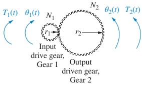
Ideal Gear Pair – Geometry and Displacement

Consider two meshed spur gears:

• Gear 1: radius \(r_1\), \(N_1\) teeth, angle \(\theta_1(t)\), torque \(T_1(t)\)
• Gear 2: radius \(r_2\), \(N_2\) teeth, angle \(\theta_2(t)\), torque \(T_2(t)\)

At the contact point, the tangential displacement must match:

\[ r_1 \theta_1 = r_2 \theta_2 \]

So the angular displacements are related by

\[ \frac{\theta_2}{\theta_1} = \frac{r_1}{r_2} = \frac{N_1}{N_2} \]

Figure 2.27: A gear system

Note

Output angle is inversely proportional to gear radius / teeth. Larger output gear → smaller output angle for the same input angle.

Clarify that we are assuming no slip and ideal gear teeth. Backlash is ignored here: mention it but emphasize we are modeling the linearized, ideal relationship. Walk through why distances along circumferences must match for meshed gears. Point out that \(N\) is proportional to circumference, hence to radius.

Ideal Gear Pair – Torque Relationship

Assume lossless gears (no energy stored or lost in the teeth). Power in = power out.

Rotational work (energy) = torque × angular displacement:

\[ T_1 \theta_1 = T_2 \theta_2 \]

Using the displacement ratio

\[ \frac{\theta_2}{\theta_1} = \frac{N_1}{N_2} \]

we get

\[ \frac{T_2}{T_1} = \frac{\theta_1}{\theta_2} = \frac{N_2}{N_1} \]

Figure 2.28: Transfer functions for lossless gears

• Angle ratio (from Gear 1 to Gear 2):

  \[ \dfrac{\theta_2}{\theta_1} = \dfrac{N_1}{N_2} \]

• Torque ratio (from Gear 1 to Gear 2):

  \[ \dfrac{T_2}{T_1} = \dfrac{N_2}{N_1} \]

Important

Gears invert the ratio:

• Smaller angle → larger torque,
• Larger angle → smaller torque.

Stress that this is like an ideal transformer: displacement and torque trade. Make sure students can interpret: a small pinion driving a large gear increases torque but reduces speed/angle. Point out that this is static relationship; dynamic effects involve inertia and damping behind each gear.

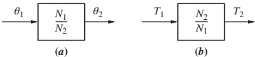
Reflecting Mechanical Impedances Through Gears

We often want to “remove” the gears from the diagram and reflect the load back to one shaft.

Consider a load inertia–damper–spring at Gear 2:

• Inertia: \(J\)
• Damping: \(D\)
• Stiffness: \(K\)

Figure 2.29: Rotational system driven by gears

From the gear relations and equations of motion, the equivalent system at \(\theta_1\) (input shaft) becomes

\[ \left[ J\left(\frac{N_1}{N_2}\right)^2 s^2 + D\left(\frac{N_1}{N_2}\right)^2 s + K\left(\frac{N_1}{N_2}\right)^2 \right] \theta_1(s) = T_1(s) \]

So each mechanical impedance term (inertia, damping, stiffness) is multiplied by \(\left(\dfrac{N_1}{N_2}\right)^2\) when reflected from Gear 2 back to Gear 1.

Walk through Figure 2.29(a) → (b) → (c): 1. Reflect input torque \(T_1\) to output using \(N_2/N_1\). 2. Write equation at the output shaft. 3. Use the angle relation \(\theta_2 = (N_1/N_2)\theta_1\) to express in terms of \(\theta_1\). Point out that all mechanical terms pick up the square of the gear ratio.

General Reflection Rule for Gears

General Rule: A rotational mechanical impedance (inertia, damping, stiffness) attached to a source shaft and reflected to a destination shaft is scaled by

\[ \left( \frac{\text{Number of teeth of gear on destination shaft}} {\text{Number of teeth of gear on source shaft}} \right)^2 \]

Equivalently, using radii \(r\):

\[ Z_\text{dest} = Z_\text{source} \left( \frac{r_\text{dest}}{r_\text{source}} \right)^2 \]

Tip

Think of gears as a mechanical impedance transformer: impedances scale with square of gear ratio, torques with first power of ratio, angles with inverse ratio.

Reinforce that “impedance” here means the coefficient that multiplies \(\theta\), \(\dot{\theta}\), or \(\ddot{\theta}\) in the Laplace domain: \(Js^2\), \(Ds\), \(K\). Give a quick numeric check (e.g., \(N_1 = 20\), \(N_2 = 40\)) so students see magnitudes.

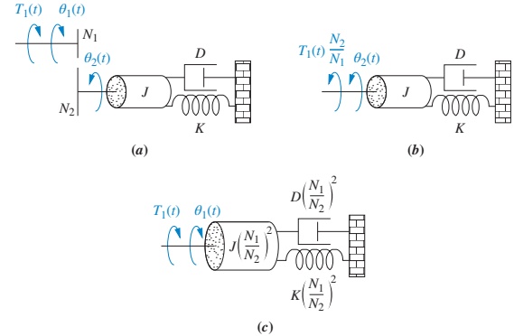
Example 2.21 – Lossless Gears: Concept

Problem: Find the transfer function \(G(s) = \dfrac{\theta_2(s)}{T_1(s)}\) for the rotational system with gears in Figure 2.30(a).

Figure 2.30: Rotational mechanical system with gears

Key ideas:

• Shafts are gear-coupled → motions are not independent → only one degree of freedom.
• We reflect all input-side elements (\(J_1, D_1, T_1\)) to the output shaft (Gear 2) to write a single equation.

Before showing equations, ask: “How many independent coordinates?” Students might initially think 2 (one for each inertia), but gears constrain motion → 1 DOF.

Example 2.21 – Lossless Gears: Reflection and Transfer Function

1. Reflect input torque and impedances to the output:

   • \(J_1\) and \(D_1\) scaled by \(\left(\dfrac{N_2}{N_1}\right)^2\)
   • \(T_1\) scaled by \(\left(\dfrac{N_2}{N_1}\right)\)

   Resulting equivalent system at \(\theta_2\):

   \[ (J_e s^2 + D_e s + K_e)\theta_2(s) = T_1(s)\frac{N_2}{N_1} \]

   where

   \[ J_e = J_1\left(\frac{N_2}{N_1}\right)^2 + J_2, \quad D_e = D_1\left(\frac{N_2}{N_1}\right)^2 + D_2, \quad K_e = K_2 \]

2. Solve for the transfer function:

   \[ G(s) = \frac{\theta_2(s)}{T_1(s)} = \frac{N_2/N_1}{J_e s^2 + D_e s + K_e} \]

   which is represented as a standard second-order system in Figure 2.30(c).

Note

The structure (second order) is familiar; the effective parameters \(J_e, D_e, K_e\) embed the gear effects.

Emphasize that the reflection step simplifies dynamics: we end up with a single inertia–damper–spring branch. Ask students: “Where does the factor \(N_2/N_1\) end up in the final transfer function?”

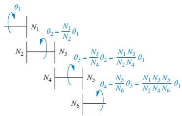
Gear Trains – Cascaded Gear Ratios

For large gear ratios, we use gear trains: multiple gear pairs in series.

Figure 2.31: Gear train

From Figure 2.31,

\[ \theta_4 = \frac{N_1 N_3 N_5}{N_2 N_4 N_6}\, \theta_1 \]

So the equivalent gear ratio from \(\theta_1\) to \(\theta_4\) is

\[ \frac{\theta_4}{\theta_1} = \prod_{k} \left( \frac{N_{\text{driver},k}}{N_{\text{driven},k}} \right) \]

Tip

For cascaded gear trains:

• Overall displacement ratio = product of individual displacement ratios.
• Impedance reflection factors use the corresponding overall ratio (squared).

Point out the analogy to cascaded electrical transformers (turns ratios multiply). Remind students to keep track of which gear is driving and which is driven at each stage.

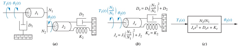
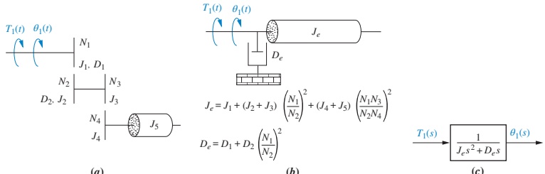
Example 2.22 – Gear Train with Losses: Concept

Problem: Find \(G(s) = \dfrac{\theta_1(s)}{T_1(s)}\) for the multi-stage gear system in Figure 2.32(a).

Figure 2.32: System using a gear train

This time:

• Gears are not lossless:
  • Gear inertias \(J_2, J_3, J_4, J_5\)
  • Damping \(D_2\) about intermediate shafts
• We want a single equation at \(\theta_1\) (input shaft).

Strategy:

• Reflect each inertia and damper to \(\theta_1\) using the appropriate gear ratios.
• Ratios are different for each element, depending on how many gear stages they cross.

Highlight that the previous example was simpler (lossless gears). Here we explicitly model inertia in the gears and friction on shafts. Key idea: each element has its own effective gear ratio relative to the reference shaft.

Example 2.22 – Gear Train with Losses: Reflection

After reflecting all impedances to \(\theta_1\):

• Equivalent inertia at input:

  \[ J_e = J_1 + (J_2 + J_3)\left(\frac{N_1}{N_2}\right)^2 + (J_4 + J_5)\left(\frac{N_1 N_3}{N_2 N_4}\right)^2 \]

• Equivalent damping at input:

  \[ D_e = D_1 + D_2\left(\frac{N_1}{N_2}\right)^2 \]

Resulting equation of motion:

\[ (J_e s^2 + D_e s)\theta_1(s) = T_1(s) \]

So the transfer function is

\[ G(s) = \frac{\theta_1(s)}{T_1(s)} = \frac{1}{J_e s^2 + D_e s} \]

Figure 2.32(b,c): Equivalent system and block diagram

Warning

Be meticulous: Each \(J\) and \(D\) may see zero, one, or two gear ratios. Compute the exact overall ratio from each element’s shaft to the reference shaft.

Walk students through one term explicitly:

• E.g., why \((J_4 + J_5)\left(\dfrac{N_1 N_3}{N_2 N_4}\right)^2\)? Because these inertias sit after two gear stages relative to \(\theta_1\). Stress that once everything is at one shaft, writing the equation is straightforward.

Skill-Assessment 2.10 – Check Your Understanding

Problem: Find the transfer function \(G(s) = \theta_2(s)/T(s)\) for the rotational mechanical system with gears shown in Figure 2.33.

Figure 2.33: Rotational mechanical system with gears

Book Answer:

\[ G(s) = \frac{1/2}{s^2 + s + 1} \]

Tip

Try to reproduce the answer by:

1. Finding the appropriate gear ratio(s).
2. Reflecting impedances to a single shaft.
3. Writing the equation of motion.
4. Solving for \(\theta_2(s)/T(s)\).

Encourage students to work this offline and then check online solutions. Remind them that pattern recognition (reflect → sum → divide) will become routine with practice.

From Mechanical to Electromechanical

So far we modeled:

• Purely mechanical rotational systems (with gears).

Now we extend to electromechanical systems:

• Electrical input (voltage, current)
• Mechanical output (shaft rotation, speed, torque)

Applications in ECE:

• Robot arm joints
• Antenna pointing systems
• Disk and tape drive actuators
• Flight simulators and haptic devices

Figure 2.34: NASA flight simulator robot arm

Emphasize that once we get a transfer function for the motor+load, we can design controllers in exactly the same way as for previous mechanical systems. Use Figure 2.34 to illustrate a sophisticated real system built up from the same building blocks.

Armature-Controlled DC Motor – Structure

• Fixed field (permanent magnet or field winding) → provides \(B\), the magnetic field.
• Armature: rotating conductor with current \(i_a(t)\) → experiences force \(F = B l i_a\).
• Torque produced turns the rotor with angle \(\theta_m(t)\) and angular speed \(\omega_m(t)\).

Two key electromagnetic relationships:

1. Torque from current:

   \[ T_m(s) = K_t I_a(s) \]

2. Back EMF from speed:

   \[ v_b(t) = K_b \frac{d\theta_m(t)}{dt} = K_b \omega_m(t) \Rightarrow V_b(s) = K_b s \theta_m(s) \]

Figure 2.35(a): DC motor schematic

Be explicit about the physical picture: moving conductor in magnetic field → both force (motor action) and induced voltage (generator action). Mention that with consistent units, \(K_t = K_b\) numerically.

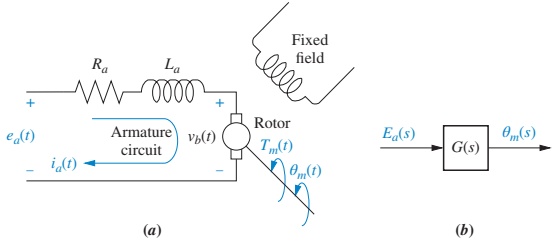
Motor Armature Circuit and Back EMF

Electrical loop around the armature:

• Armature resistance: \(R_a\)
• Armature inductance: \(L_a\)
• Back EMF: \(V_b(s)\)
• Applied voltage: \(E_a(s)\)

Kirchhoff’s voltage law:

\[ R_a I_a(s) + L_a s I_a(s) + V_b(s) = E_a(s) \]

Substitute \(V_b(s) = K_b s \theta_m(s)\) and \(I_a(s) = \dfrac{1}{K_t} T_m(s)\) to couple the electrical and mechanical domains.

Note

The back EMF \(V_b\) acts like a negative feedback in the motor:

• Faster rotation → larger \(V_b\) → reduces armature current → limits torque.

Explain that this is why DC motors naturally resist sudden load changes to some extent: the back EMF changes current. Prepare students to plug in the mechanical dynamics next.

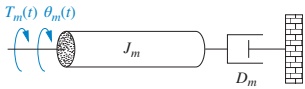
Mechanical Loading of the Motor

Mechanical side (shaft dynamics):

Figure 2.36: Typical equivalent mechanical loading

• Equivalent inertia at armature: \(J_m\)
• Equivalent viscous damping: \(D_m\)

Equation in Laplace domain:

\[ T_m(s) = (J_m s^2 + D_m s)\, \theta_m(s) \]

This \(J_m\) and \(D_m\) include both:

• Motor’s own inertia and damping.
• Load inertia and damping reflected through gear(s) to the armature shaft.

Connect back to earlier gear reflection: \(J_m\) and \(D_m\) are computed using those formulas. This unifies mechanical modeling with the electrical motor model.

DC Motor Transfer Function (Neglecting Armature Inductance)

Substitute \(T_m(s)\) and \(V_b(s)\) into the armature KVL, assuming \(L_a\) is small:

1. Start with

   \[ \frac{(R_a + L_a s)T_m(s)}{K_t} + K_b s \theta_m(s) = E_a(s) \]

2. With \(L_a \approx 0\):

   \[ \frac{R_a}{K_t} T_m(s) + K_b s \theta_m(s) = E_a(s) \]

3. Use \(T_m(s) = (J_m s^2 + D_m s)\theta_m(s)\):

   \[ \left[\frac{R_a}{K_t} (J_m s^2 + D_m s) + K_b s \right]\theta_m(s) = E_a(s) \]

Rearrange:

\[ \left[\frac{R_a}{K_t} (J_m s + D_m) + K_b \right] s \theta_m(s) = E_a(s) \]

So the transfer function is

\[ \frac{\theta_m(s)}{E_a(s)} = \frac{K_t/(R_a J_m)}{s\left[s + \frac{1}{J_m} \left(D_m + \frac{K_t K_b}{R_a}\right)\right]} \]

or in simplified form

\[ \frac{\theta_m(s)}{E_a(s)} = \frac{K}{s(s + \alpha)} \]

Important

A DC motor (with this approximation) behaves like:

• One integrator (from speed to position), and
• One stable first-order pole (electromechanical time constant).

Interpret \(K\) as the static gain from voltage to position velocity integrated. Interpret \(\alpha\) as related to the effective damping: larger \(D_m\) or stronger electrical damping (large \(K_t K_b/R_a\)) → faster \(\alpha\) (shorter time constant).

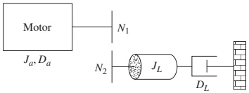
Including the Gear and Load – Effective \(J_m\) and \(D_m\)

Consider a motor with armature inertia \(J_a\) and damping \(D_a\), driving a load of inertia \(J_L\) and damping \(D_L\) through a gear pair with ratio \(N_1:N_2\) (armature:load):

Figure 2.37: DC motor driving a rotational mechanical load

Reflect \(J_L\) and \(D_L\) to the armature:

\[ J_m = J_a + J_L\left(\frac{N_1}{N_2}\right)^2 \]

\[ D_m = D_a + D_L\left(\frac{N_1}{N_2}\right)^2 \]

Use these \(J_m\) and \(D_m\) in the DC motor transfer function

\[ \frac{\theta_m(s)}{E_a(s)} = \frac{K_t/(R_a J_m)}{s\left[s + \frac{1}{J_m} \left(D_m + \frac{K_t K_b}{R_a}\right)\right]} \]

Ask: “What happens to \(J_m\) if we use a large gear reduction (\(N_1 \ll N_2\))?” → The reflected load inertia shrinks significantly, which is one reason high gear ratios are helpful when driving heavy loads.

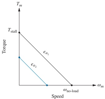
Determining Electrical Constants via Torque–Speed Curves

Start from the DC motor steady-state equation (with \(L_a=0\)):

\[ \frac{R_a}{K_t}T_m(s) + K_b s \theta_m(s) = E_a(s) \]

Inverse Laplace and assume DC (steady-state) operation:

\[ \frac{R_a}{K_t}T_m + K_b \omega_m = e_a \]

Solve for torque:

\[ T_m = -\frac{K_b K_t}{R_a}\omega_m + \frac{K_t}{R_a} e_a \]

This is a straight line in the torque–speed plane:

• Intercept at \(\omega_m = 0\): stall torque

  \[ T_{\text{stall}} = \frac{K_t}{R_a}e_a \]

• Intercept at \(T_m = 0\): no-load speed

  \[ \omega_{\text{no-load}} = \frac{e_a}{K_b} \]

Thus

\[ \frac{K_t}{R_a} = \frac{T_{\text{stall}}}{e_a}, \quad K_b = \frac{e_a}{\omega_{\text{no-load}}} \]

Figure 2.38: Torque–speed curves

Tip

A dynamometer test (measuring stall torque and no-load speed for a given \(e_a\)) gives the motor constants needed in the transfer function.

Emphasize that this is practical: in lab or data sheets, motors are often specified by stall torque and no-load speed. Relate to Virtual Experiment 2.2.

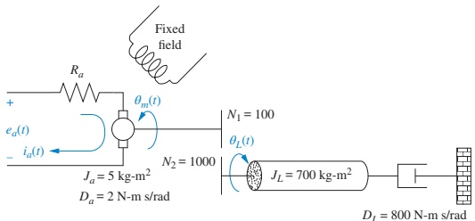
Example 2.23 – DC Motor and Load

Problem: Given the DC motor, load, gear ratio, and torque–speed curve in Figure 2.39, find \(G(s) = \dfrac{\theta_L(s)}{E_a(s)}\).

Figure 2.39: DC motor and load

Example 2.23 – DC Motor and Load

Step 1: Mechanical Constants

From the data:

\[ J_m = J_a + J_L\left(\frac{N_1}{N_2}\right)^2 = 5 + 700\left(\frac{1}{10}\right)^2 = 12 \]

\[ D_m = D_a + D_L\left(\frac{N_1}{N_2}\right)^2 = 2 + 800\left(\frac{1}{10}\right)^2 = 10 \]

From the torque–speed curve:

• Stall torque: \(T_{\text{stall}} = 500\)
• No-load speed: \(\omega_{\text{no-load}} = 50\)
• Input voltage: \(e_a = 100\)

Pause to check units (e.g., N·m·s/rad for damping, kg·m² for inertia). Emphasize again the square of the gear ratio.

Example 2.23 – DC Motor and Load

Then

\[ \frac{K_t}{R_a} = \frac{T_{\text{stall}}}{e_a} = \frac{500}{100} = 5 \]

\[ K_b = \frac{e_a}{\omega_{\text{no-load}}} = \frac{100}{50} = 2 \]

Plug into the motor transfer function:

\[ \frac{\theta_m(s)}{E_a(s)} = \frac{5/12}{s\left\{s + \frac{1}{12}[10 + (5)(2)]\right\}} = \frac{0.417}{s(s + 1.667)} \]

Use gear ratio \(\dfrac{N_1}{N_2} = \dfrac{1}{10}\) to get load angle:

\[ \frac{\theta_L(s)}{E_a(s)} = \frac{0.0417}{s(s + 1.667)} \]

Figure 2.39(c): Block diagram

Note

Notice: The poles (dynamics) do not change with this simple gear scaling; the gear changes only the output gain between \(\theta_m\) and \(\theta_L\).

Clarify that, strictly, changing gear ratio would change \(J_m\) and \(D_m\), thus affecting poles. Here, the ratio used in reflecting load and the ratio used for angle appear separately, but we’re using the specific given data, so the final dynamics come out as shown.

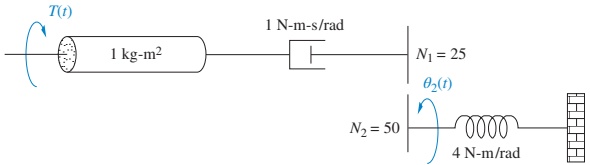
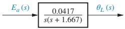
Skill-Assessment 2.11 – Motor + Gear + Load

Problem: For the electromechanical system shown in Figure 2.40, with torque–speed curve

\[ T_m = -8\omega_m + 200 \]

at \(e_a = 100\ \text{V}\), find

\[ G(s) = \frac{\theta_L(s)}{E_a(s)} \]

Figure 2.40: Electromechanical system

Answer:

\[ G(s) = \frac{1/20}{s\left[s + \dfrac{15}{2}\right]} \]

Tip

To solve:

1. Extract \(K_t/R_a\) and \(K_b\) from the torque–speed relation.
2. Reflect load inertia/damping through gears to find \(J_m\) and \(D_m\).
3. Use the DC motor transfer function formula.
4. Include gear ratio between motor and load angles.

Point out that this is essentially the same workflow as Example 2.23, but as a self-check. Encourage students to verify each step symbolically before plugging numbers.

Electric Circuit Analogs

Mechanical → Electrical analogs:

• Let us reuse circuit intuition and tools (nodal/mesh analysis, SPICE simulation).
• Reveal deep similarities between energy-storage systems across domains.
• Provide alternative ways to derive equations of motion.

Two main types:

1. Series analog (mesh equations ↔︎ equations of motion in velocity).
2. Parallel analog (nodal equations ↔︎ equations of motion in velocity).

Figure 2.41 and 2.43: Mechanical system and analogs

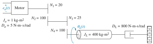
Motivate by saying: If you are stronger in circuits than in mechanics, analogs can make mechanical modeling easier. Also, analogs appear historically in early analog computers, which solved differential equations using electrical networks.

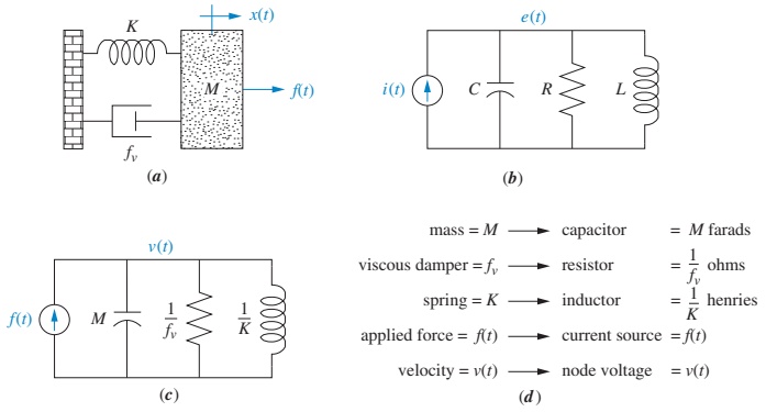
Series Analog – Single Mass–Spring–Damper

Equation of motion (Laplace, displacement):

\[ (M s^2 + f_v s + K) X(s) = F(s) \]

To match with current-based mesh equations, rewrite in terms of velocity \(V(s) = s X(s)\):

\[ \left(M s + f_v + \frac{K}{s}\right) V(s) = F(s) \]

Electrical series RLC mesh:

\[ (L s + R + \frac{1}{C s}) I(s) = E(s) \]

Analog mapping (series type):

• Velocity \(V(s)\) ↔︎ Current \(I(s)\)
• Force \(F(s)\) ↔︎ Voltage \(E(s)\)
• Mass \(M\) ↔︎ Inductance \(L\)
• Viscous damping \(f_v\) ↔︎ Resistance \(R\)
• Spring constant \(K\) ↔︎ Inverse of capacitance \(1/C\)

Note

In a series analog, mechanical impedances map onto series electrical impedances.

Students often confuse which quantity maps to current vs. voltage. Stress: here, velocity ↔︎ current because both appear multiplied by total impedance in the equations.

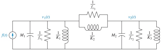
Series Analog – Multi-Mass System (Example 2.24)

Problem: Draw a series analog for the mechanical system of Figure 2.17(a).

Mechanical equations (after converting to velocity):

\[ \left[M_1 s + (f_{v_1}+f_{v_3}) + \frac{K_1+K_2}{s}\right]V_1(s) - \left(f_{v_3}+\frac{K_2}{s}\right)V_2(s) = F(s) \]

\[ -\left(f_{v_3}+\frac{K_2}{s}\right)V_1(s) + \left[M_2 s+(f_{v_2}+f_{v_3})+\frac{K_2+K_3}{s}\right]V_2(s) = 0 \]

Coefficients correspond to sums of series impedances:

• Impedances tied to motion of \(M_1\) → first mesh.
• Impedances between \(M_1\) and \(M_2\) → shared between both meshes.
• Impedances tied to \(M_2\) → second mesh.

Result:

Figure 2.42: Series analog

Point out which inductor, resistor, capacitor corresponds to each mechanical element. This reinforces the mapping in a more complex context.

Parallel Analog – Single Mass–Spring–Damper

Now we match with nodal equations instead of mesh equations.

Electrical parallel RLC node:

\[ \left(C s + \frac{1}{R} + \frac{1}{L s}\right) E(s) = I(s) \]

Mechanical equation in velocity form:

\[ \left(M s + f_v + \frac{K}{s}\right) V(s) = F(s) \]

If we identify - Velocity \(V(s)\) ↔︎ Voltage \(E(s)\) - Force \(F(s)\) ↔︎ Current \(I(s)\) then

• \(M\) ↔︎ \(1/L\) (since \(1/(L s)\) term aligns with mass term when seen as admittance)
• \(f_v\) ↔︎ \(1/R\)
• \(K\) ↔︎ \(C\)

Figure 2.43: Parallel analog

Note

In a parallel analog, - Velocity ↔︎ voltage, - Force ↔︎ current, - Mechanical admittances map onto electrical admittances.

Clarify that the mapping is different from the series analog, but both are valid. Choice depends on whether you prefer mesh or nodal methods, or on the type of circuit simulator used.

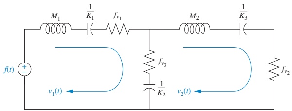
Parallel Analog – Multi-Mass System (Example 2.25)

Problem: Draw a parallel analog for the mechanical system of Figure 2.17(a).

Starting from the same mechanical equations (in velocity form), interpret each coefficient as a sum of admittances:

• Admittances associated with \(M_1\) connect to node 1.
• Admittances between \(M_1\) and \(M_2\) connect between node 1 and node 2.
• Admittances associated with \(M_2\) connect to node 2.

Resulting parallel analog:

Figure 2.44: Parallel analog

Highlight that the graph structure (two nodes plus interconnection admittance) closely mirrors the mechanical layout of two masses and a coupling spring/damper.

Skill-Assessment 2.12 – Rotational Analogs

Problem: Draw a series and parallel analog for the rotational mechanical system of Figure 2.22.

(Hint: use rotational analogs of mass, damping, spring: inertia \(J\), viscous damping \(D\), torsional stiffness \(K\).)

Answer available online.

Tip

Workflow:

1. Write equations of motion in Laplace domain.
2. Convert to angular velocity (if needed).
3. Match with either mesh (series analog) or nodal (parallel analog) equations.
4. Map each rotational element to an R, L, or C appropriately.

Encourage students to note symmetry with translational analogs: equations look the same with \(\theta\) instead of \(x\), \(T\) instead of \(F\), \(J\) instead of \(M\), etc.

Summary / Key Points

• Gears:
  • \(\dfrac{\theta_2}{\theta_1} = \dfrac{N_1}{N_2}\), \(\dfrac{T_2}{T_1} = \dfrac{N_2}{N_1}\).
  • Mechanical impedances reflect through gears with the square of gear ratio.
  • Gear trains multiply individual ratios to get an overall ratio.
• Rotational systems with gears:
  • Reflect all load impedances to a single shaft; then write one equation of motion.
  • Transfer functions look like standard 1st or 2nd order forms with effective \(J\), \(D\), \(K\).
• DC motor modeling:
  • Electrical: \(R_a I_a + L_a s I_a + K_b s \theta_m = E_a\).
  • Mechanical: \(T_m = (J_m s^2 + D_m s)\theta_m\), \(T_m = K_t I_a\).
  • Combined TF (ignoring \(L_a\)): \(\dfrac{\theta_m}{E_a} = \dfrac{K_t/(R_a J_m)}{s\left[s + \dfrac{1}{J_m}\left(D_m + \dfrac{K_t K_b}{R_a}\right)\right]}\).

• Torque–speed curves:
  • Provide \(K_t/R_a\) and \(K_b\) via stall torque and no-load speed.
• Electric circuit analogs:
  • Series analog: velocity ↔︎ current, force ↔︎ voltage; impedances in series.
  • Parallel analog: velocity ↔︎ voltage, force ↔︎ current; admittances in parallel.

Use this slide to connect all topics: gears → reflected impedances → DC motor with load → circuit analogs. Highlight how transfer function derivation is systematic: 1. Write physics-based equations. 2. Reflect through gears if needed. 3. Solve for output over input in Laplace domain.

Formula Summary

Gear relationships (ideal, lossless):

• Displacement ratio:

  \[ \frac{\theta_2}{\theta_1} = \frac{r_1}{r_2} = \frac{N_1}{N_2} \]

• Torque ratio:

  \[ \frac{T_2}{T_1} = \frac{\theta_1}{\theta_2} = \frac{N_2}{N_1} \]

• Impedance reflection (source → destination):

  \[ Z_\text{dest} = Z_\text{source} \left( \frac{\text{teeth at destination shaft}} {\text{teeth at source shaft}} \right)^2 \]

Gear train overall ratio:

\[ \theta_\text{out} = \left(\prod_k \frac{N_{\text{driver},k}}{N_{\text{driven},k}}\right)\theta_\text{in} \]

DC motor relationships:

• Back EMF:

  \[ v_b(t) = K_b \omega_m(t), \quad V_b(s) = K_b s \theta_m(s) \]

• Torque–current:

  \[ T_m(s) = K_t I_a(s) \]

• Armature circuit (Laplace):

  \[ R_a I_a(s) + L_a s I_a(s) + K_b s \theta_m(s) = E_a(s) \]

• Mechanical load at armature:

  \[ T_m(s) = (J_m s^2 + D_m s)\theta_m(s) \]

• Effective inertia/damping (with gear ratio \(N_1:N_2\)):

  \[ J_m = J_a + J_L\left(\frac{N_1}{N_2}\right)^2, \quad D_m = D_a + D_L\left(\frac{N_1}{N_2}\right)^2 \]

• Transfer function (neglect \(L_a\)):

  \[ \frac{\theta_m(s)}{E_a(s)} = \frac{K_t/(R_a J_m)}{s\left[s + \frac{1}{J_m} \left(D_m + \frac{K_t K_b}{R_a}\right)\right]} \]

Torque–speed curve quantities:

• Stall torque:

  \[ T_{\text{stall}} = \frac{K_t}{R_a} e_a \]

• No-load speed:

  \[ \omega_{\text{no-load}} = \frac{e_a}{K_b} \]

• Electrical constants:

  \[ \frac{K_t}{R_a} = \frac{T_{\text{stall}}}{e_a}, \quad K_b = \frac{e_a}{\omega_{\text{no-load}}} \]

Electric analog mappings (summary):

• Series analog (mesh):

  • Velocity \(V\) ↔︎ Current \(I\)
  • Force \(F\) ↔︎ Voltage \(E\)
  • \(M\) ↔︎ \(L\), \(f_v\) ↔︎ \(R\), \(K\) ↔︎ \(1/C\)

• Parallel analog (node):

  • Velocity \(V\) ↔︎ Voltage \(E\)
  • Force \(F\) ↔︎ Current \(I\)
  • \(M\) ↔︎ \(1/L\), \(f_v\) ↔︎ \(1/R\), \(K\) ↔︎ \(C\)

Encourage students to keep this formula sheet handy while working on problem sets involving gears and DC motors.

Interactive

Using This Interactive Deck

• This addendum lets you experiment with gears, DC motors, and analogs using live Python (Pyodide) and Observable JS (OJS) directly in the browser.
• You can:
  • Change gear tooth counts and see how angles and torques change.
  • Explore how reflected inertia changes with gear ratio.
  • Visualize DC motor step responses as you vary parameters.
  • See how motor torque–speed lines depend on motor constants.

Tip

Change the sliders and code, then click Run Code in the Python cells to see how the system behavior changes in real time.

Explain to students that this deck is meant for experimentation, not just passive viewing. Emphasize that they don’t need a local Python installation; everything runs in the browser via Pyodide.

1. Interactive Code – Gear Ratios (Static Relationships)

Play with the basic gear formulas:

• \(\displaystyle \frac{\theta_2}{\theta_1} = \frac{N_1}{N_2}\)
• \(\displaystyle \frac{T_2}{T_1} = \frac{N_2}{N_1}\)

Note

Try:

• Make \(N_1 < N_2\) (gear reduction).
• Make \(N_1 > N_2\) (gear up). Observe how angle and torque ratios swap.

Encourage students to interpret the printed ratios physically. Ask: what does it mean if \(T_2/T_1 = 2\) but \(\theta_2/\theta_1 = 0.5\)?

2. Reactive Visualization – Gear Impedance Reflection

We know that when reflecting a load inertia \(J_L\) through a gear ratio,

\[ J_\text{reflected} = J_L \left(\frac{N_\text{dest}}{N_\text{source}}\right)^2 \]

Use the sliders to see how reflected inertia changes with gear ratio.

viewof N_source = Inputs.range([5, 100], {step: 1, label: "N_source (source shaft teeth)"})
viewof N_dest   = Inputs.range([5, 100], {step: 1, label: "N_dest (destination shaft teeth)"})
viewof J_L      = Inputs.range([0.01, 10], {step: 0.01, label: "Load inertia J_L (kg·m²)"})

Tip

Interpretation:

• Fix \(J_L\) and \(N_\text{source}\), vary \(N_\text{dest}\).
• Larger \(N_\text{dest}\) (bigger gear at destination) → larger reflected inertia at the source.

Point out that this explains why high reductions can make the motor “feel” a lighter or heavier load depending on direction of reflection.

3. Interactive Code – Gear Train Overall Ratio

Experiment with a 3-stage gear train like in Figure 2.31.

We use

\[ \theta_4 = \frac{N_1 N_3 N_5}{N_2 N_4 N_6} \theta_1 \]

Note

Modify the \(N\) values to see how cascading several modest ratios can create a large overall reduction.

You can ask students: what combination of modest stage ratios gives about 100:1 total reduction? This ties to practical gear train design in robotics.

4. Reactive DC Motor – Step Response vs. Parameters

We model the DC motor (position output) as

\[ \frac{\theta_m(s)}{E_a(s)} = \frac{K}{s(s + \alpha)} \]

where

• \(K = \dfrac{K_t}{R_a J_m}\)
• \(\alpha = \dfrac{1}{J_m}\left(D_m + \dfrac{K_t K_b}{R_a}\right)\)

Use sliders to vary \(K\) and \(\alpha\) and see the step response.

viewof K_gain   = Inputs.range([0.01, 1], {step: 0.01, label: "K (position gain)"})
viewof alpha    = Inputs.range([0.1, 10], {step: 0.1, label: "α (1/s)"})
viewof t_final  = Inputs.range([1, 10], {step: 0.5, label: "Simulation time (s)"})

Tip

Observations:

• Larger \(\alpha\) → faster response (more damping/electrical braking).
• Larger \(K\) → greater steady-state slope (more motion per volt).

Relate \(\alpha\) changes to increasing \(D_m\) or electrical damping \(\frac{K_t K_b}{R_a}\). Ask students to find parameter pairs that yield an overshoot-free, “fast enough” response.

5. Reactive DC Motor – Torque–Speed Line Explorer

We derived the steady-state torque–speed relationship:

\[ T_m = -\frac{K_b K_t}{R_a}\,\omega_m + \frac{K_t}{R_a} e_a \]

Use sliders to vary \(K_t/R_a\), \(K_b\), and \(e_a\) and see the line.

viewof Kt_over_Ra = Inputs.range([0.1, 10], {step: 0.1, label: "K_t / R_a"})
viewof Kb         = Inputs.range([0.1, 10], {step: 0.1, label: "K_b"})
viewof Ea_dc      = Inputs.range([10, 200], {step: 10, label: "Applied voltage e_a (V)"})

Note

Questions to explore:

• What happens to the line if you double \(e_a\)?
• How does increasing \(K_b\) (stronger back EMF) change no-load speed and slope?
• How does increasing \(K_t/R_a\) change stall torque?

Connect this back to Example 2.23: identify \(T_{\text{stall}}\) and \(\omega_{\text{no-load}}\) from a given line and recover \(K_t/R_a\) and \(K_b\).

6. Interactive Code – Compute \(J_m\) and \(D_m\) with Gears

Given

\[ J_m = J_a + J_L\left(\frac{N_1}{N_2}\right)^2, \quad D_m = D_a + D_L\left(\frac{N_1}{N_2}\right)^2 \]

experiment with different gear ratios and load values.

Tip

Try changing \(N_1/N_2\) to 1/5, 1/10, 1/20, etc. Observe how \(J_m\) and \(D_m\) scale with the square of the gear ratio.

Encourage students to reflect: a higher reduction (smaller \(N_1/N_2\)) “lightens” the load as seen by the motor. This is crucial when selecting a motor for a heavy robotic joint.

7. Reactive – First-Order Mechanical Load via Gear Ratio

We can visualize how gear ratio affects a first-order load dynamics in angle:

\[ G(s) = \frac{\theta(s)}{T(s)} = \frac{1}{J_\text{eff} s^2 + D_\text{eff} s} \]

where \(J_\text{eff}, D_\text{eff}\) depend on gear ratio.

viewof N1_slider = Inputs.range([1, 20], {step: 1, label: "N1 (motor gear teeth)"})
viewof N2_slider = Inputs.range([1, 50], {step: 1, label: "N2 (load gear teeth)"})
viewof JL_slider = Inputs.range([10, 1000], {step: 10, label: "Load inertia J_L"})
viewof DL_slider = Inputs.range([10, 1000], {step: 10, label: "Load damping D_L"})

Warning

This is a rough approximation, but it illustrates:

• Larger reflected \(J_m\) → slower angle response.
• Larger reflected \(D_m\) → more damping, shorter transient.

Make it clear that the model here is simplified for pedagogy. The key point is qualitative: gear ratio shapes the effective inertia/damping and thus the time response.

8. Interactive – Series Analog Parameter Mapping

Recall series analog mapping (single-DOF translational):

• \(M\) ↔︎ \(L\), \(f_v\) ↔︎ \(R\), \(K\) ↔︎ \(1/C\)

Try mapping a given mechanical system to RLC values.

Note

Modify \(M\), \(f_v\), and \(K\). Think about how a heavier mass translates to larger inductance, and stiffer spring to a smaller capacitance.

You can ask students: if you double the mass, which electrical parameter doubles? If you want to simulate a very stiff spring, what happens to \(C\)?

9. Reactive – Parallel Analog Admittance Matching

For the parallel analog, the mapping is (single-DOF):

• \(M\) ↔︎ \(1/L\), \(f_v\) ↔︎ \(1/R\), \(K\) ↔︎ \(C\)

Use sliders to see electrical parameters for a given mechanical system.

viewof M_mech   = Inputs.range([0.5, 10], {step: 0.5, label: "Mass M"})
viewof fv_mech  = Inputs.range([0.5, 10], {step: 0.5, label: "Damping f_v"})
viewof K_mech   = Inputs.range([5, 200], {step: 5, label: "Stiffness K"})

Tip

Compare this to the series analog mapping:

• Here, mass → inverse inductance; in series analog, mass → inductance. This is why we call this an admittance-based (parallel) analog.

Highlight that both analogs are mathematically valid; the choice is driven by convenience and the desired circuit topology.

10. Wrap-Up – What to Try Next

To deepen your understanding, try these mini-challenges in this deck:

1. Gear design exercise:
   • Choose a target overall ratio (e.g., 50:1) and find a 3-stage gear train with modest ratios whose product is near 50.
   • Use the gear train code to confirm \(\theta_\text{out}/\theta_\text{in}\).
2. Motor selection exercise:
   • Use the torque–speed explorer: pick \(K_t/R_a\), \(K_b\), \(e_a\) to achieve a desired stall torque and no-load speed.
3. Load matching exercise:
   • For a heavy load (\(J_L\) large), adjust \(N_1/N_2\) to make \(J_m\) small enough that the motor response is “fast,” but not so small that back-driving becomes impossible.
4. Analog modeling exercise:
   • Map a two-mass mechanical system to both series and parallel analogs (on paper), then use the mapping code to check individual parameter conversions.

Important

Use these interactive tools as a sandbox: change parameters, observe results, and connect them back to the equations in the main lecture. This is how theory becomes engineering intuition.

Encourage students to save or screenshot parameter settings that produce interesting behaviors (e.g., critically damped, underdamped). Suggest they re-derive the associated time-domain or frequency-domain behavior analytically as practice.