Translational & Rotational Mechanical System Transfer Functions

Control 2.3

Imron Rosyadi

Translational & Rotational Mechanical System Transfer Functions

Chapter 2.5–2.6

This deck is meant for one 50–75 minute lecture. The flow is:

1. Remind students what a transfer function is from electrical circuits.
2. Build mechanical analogies (spring–damper–mass).
3. Do 1‑DOF translational example and introduce mechanical impedance.
4. Move to multi‑DOF translational systems, show “mesh‑like” equation pattern.
5. Quick practice problem.
6. Repeat the same ideas for rotational systems.
7. End with summary and formula “cheat sheet”.

Encourage students to “see” mechanical systems as circuits: same algebra, different physical meaning.

Learning Objectives

By the end of this session, you should be able to:

1. Write equations of motion for translational and rotational mechanical systems using Newton’s laws.
2. Derive transfer functions \(G(s)\) relating displacement (or angle) to applied force (or torque).
3. Use the concept of mechanical impedance to write equations directly in the \(s\)‑domain without first writing time‑domain differential equations.
4. Recognize and exploit the electrical–mechanical analogies (R, L, C ↔︎ damper, mass, spring).
5. Write equations of motion for multi‑degree‑of‑freedom systems by inspection, using “mesh‑like” patterns.

Stress that the algebra they already know from circuits is now being “reused” in mechanics. The key new ideas: - Mechanical impedance \(Z_M(s) = F(s)/X(s)\) or \(T(s)/\theta(s)\). - Degrees of freedom (DOF) and how they map to number of equations. - Two big analogies: - Force–Voltage / Velocity–Current (“mesh” style) - Force–Current / Velocity–Voltage (“node” style, mentioned but not used here).

Big Picture: Why We Care

Control systems in ECE often involve mechanics:

• Hard disk drive head positioning (rotational + translational).
• 3D printer or CNC axis control.
• Automotive suspensions (sprung mass).
• Robotics joints with flexible couplings.

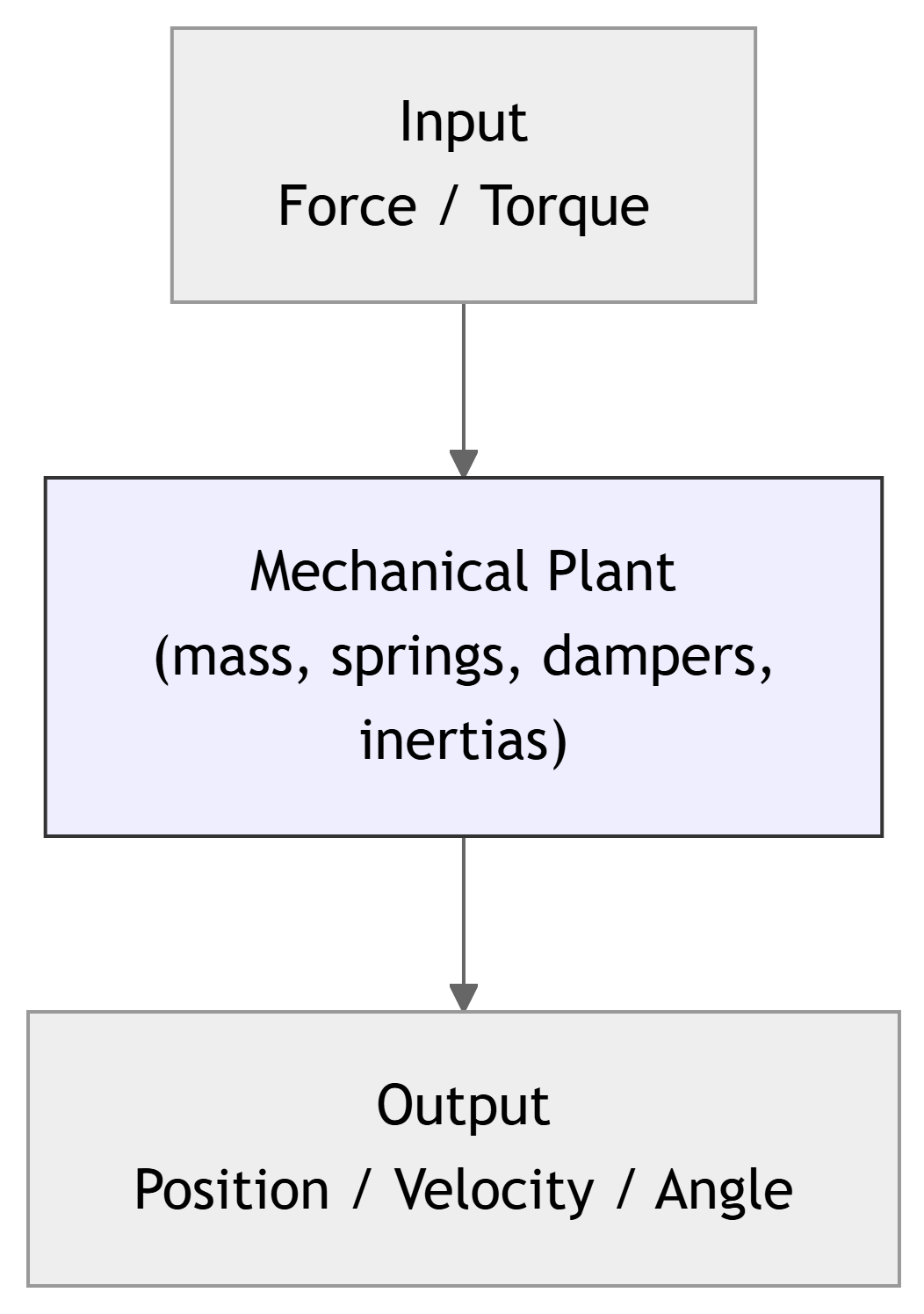
To design controllers, we need transfer functions that describe how motion responds to forces/torques.

Tip

We will show that mechanical systems can be modeled just like electrical RLC circuits, enabling us to reuse circuit techniques.

Connect this to their intuition: cars bouncing, drones tilting, motors driving loads. Emphasize: once we have \(G(s)\), all the Laplace/transfer function tools (stability, step responses, Bode plots) become available.

Review: Transfer Functions

For any linear time-invariant (LTI) system with zero initial conditions:

\[ G(s) = \frac{Y(s)}{U(s)} \]

where

• \(U(s)\) = Laplace transform of input
• \(Y(s)\) = Laplace transform of output

In circuits, examples:

• \(G(s) = \dfrac{V_{\text{out}}(s)}{V_{\text{in}}(s)}\)
• \(G(s) = \dfrac{I_{\text{out}}(s)}{V_{\text{in}}(s)}\)

In mechanical systems, we will see examples like:

• \(G(s) = \dfrac{X(s)}{F(s)}\) (displacement per force)
• \(G(s) = \dfrac{\theta(s)}{T(s)}\) (angle per torque)

Remind them that the procedure is: 1. Write differential equation(s) from physics. 2. Laplace transform (zero ICs). 3. Solve algebraically for output over input to get \(G(s)\).

We now do this for mechanical systems.

Translational Mechanical Elements

Three basic translational elements

1. Spring (stiffness \(K\))
2. Viscous damper (damping coefficient \(f_v\))
3. Mass (\(M\))

Variables:

• Force: \(f(t)\) [N]
• Displacement: \(x(t)\) [m]
• Velocity: \(v(t) = \dfrac{dx}{dt}\) [m/s]

![images/chapter_2/Pasted%20image%2020260221134345.png){height=170}

If the images don’t show, verbally describe: - Spring exerts force proportional to displacement. - Damper exerts force proportional to relative velocity (like a shock absorber). - Mass resists acceleration (inertia).

Mention SI units explicitly to reinforce physical meaning.

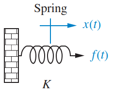
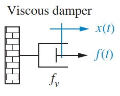
Translational Element Equations (Time Domain)

Table 2.4 (time-domain relations)

Component	Force–velocity	Force–displacement
Spring	\(f(t) = K \displaystyle\int_{0}^{t} v(\tau)\, d\tau\)	\(f(t) = K x(t)\)
Viscous damper	\(f(t) = f_v v(t)\)	\(f(t) = f_v \dfrac{dx(t)}{dt}\)
Mass	\(f(t) = M \dfrac{dv(t)}{dt}\)	\(f(t) = M \dfrac{d^2 x(t)}{dt^2}\)

Units recap:

• \(f(t)\) – N (newtons)
• \(x(t)\) – m (meters)
• \(v(t)\) – m/s
• \(K\) – N/m
• \(f_v\) – N·s/m
• \(M\) – kg (= N·s²/m)

Emphasize two equivalent descriptions:

• In terms of velocity (left column) – closer to circuit analogies where current is “rate of charge”.
• In terms of displacement (right column) – more convenient because we often care about position.

We will primarily work with displacement-based equations.

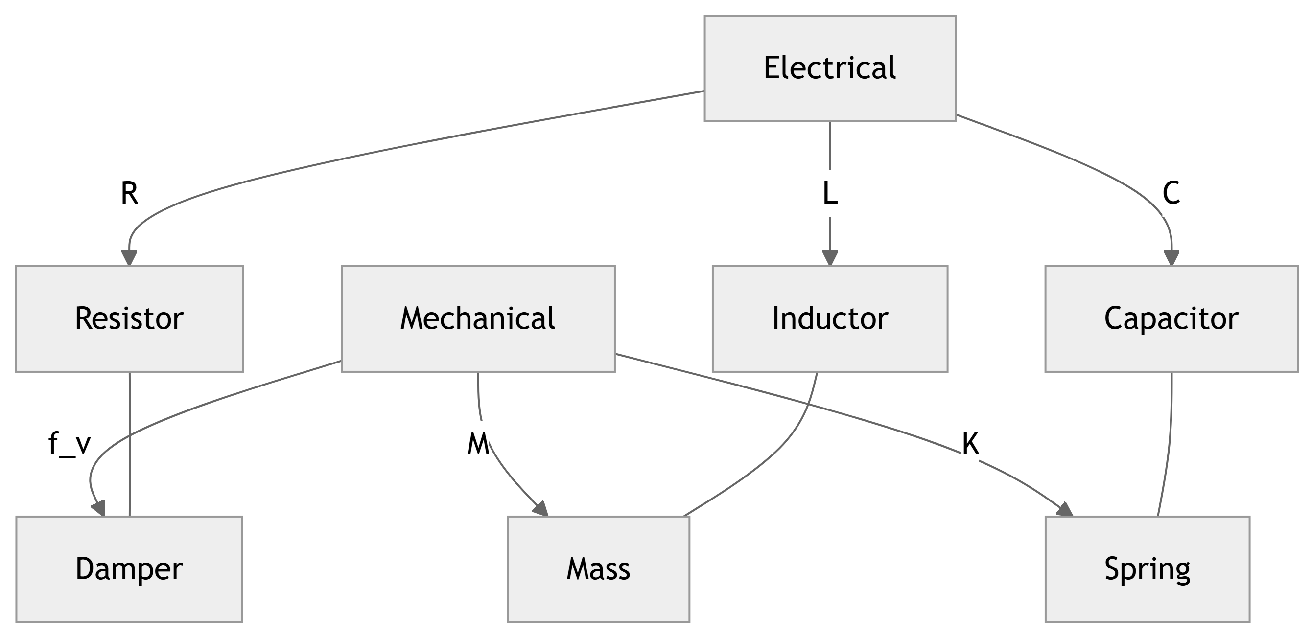
Electrical–Mechanical Analogies (Mesh-Style)

From comparing mechanical and electrical tables:

• Mechanical force \(f\) ↔︎ Electrical voltage \(v\)
• Mechanical velocity \(v\) ↔︎ Electrical current \(i\)
• Mechanical displacement \(x\) ↔︎ Electrical charge \(q\)

Element analogies (this “mesh-style” view):

• Spring ↔︎ Capacitor
• Viscous damper ↔︎ Resistor
• Mass ↔︎ Inductor

Implication:

• Summing forces (in terms of velocity) ↔︎ Summing voltages (in terms of current)
• Equations look like mesh equations in circuits.

Note

There is also a force–current analogy (node-style), but in this section we mainly use the force–voltage analogy.

Clarify: “analogous” means the equations look the same, not that the physics are identical. The analogy is useful for reusing circuit methods (mesh equations, impedances, etc.).

1‑DOF Translational System: Physical Setup

Consider the system in Figure 2.15(a):

• A mass \(M\) attached to a fixed wall by a spring (\(K\)) and a damper (\(f_v\)) in parallel.
• An external force \(f(t)\) is applied to the mass.
• We measure the mass displacement \(x(t)\).

Goal: Find transfer function \(G(s) = \dfrac{X(s)}{F(s)}\).

Steps:

1. Draw a free-body diagram (FBD).
2. Apply Newton’s 2nd law (sum of forces = mass × acceleration).
3. Write the equation of motion.
4. Laplace transform and solve for \(G(s)\).

Figure 2.15(a): Mass–spring–damper system

Remind them: pick a positive direction (to the right). All forces acting on the mass in that direction are positive; opposing forces are negative.

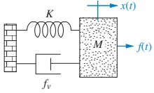
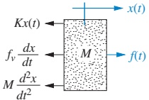
1‑DOF Translational: Free-Body Diagram

Figure 2.16(a): Free-body diagram

For motion assumed to the right:

• Applied force \(f(t)\) acts to the right.
• Spring force \(Kx(t)\) acts left (restoring).
• Damper force \(f_v \dfrac{dx}{dt}\) acts left (opposes motion).
• Inertial force \(M \dfrac{d^2x}{dt^2}\) (mass × acceleration) effectively appears on left side of the equation.

Equation from Newton’s law (sum of forces = \(M\ddot{x}\)):

\[ M\frac{d^{2}x(t)}{dt^{2}}+f_{v}\frac{dx(t)}{dt}+Kx(t)=f(t) \]

Show sign reasoning explicitly:

• Write \(\Sigma f = M \ddot{x}\) with directions.
• Rearranged, this yields “all impedance-like terms times \(x(t)\) equals applied force”.

This is their first “mechanical differential equation of motion” in the course.

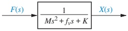
1‑DOF Translational: Transfer Function

Take Laplace transform with zero initial conditions:

\[ M s^{2}X(s)+f_{v}s X(s)+K X(s)=F(s) \]

Factor \(X(s)\):

\[ (M s^{2}+f_{v}s+K)X(s)=F(s) \]

Transfer function:

\[ G(s) = \frac{X(s)}{F(s)}=\frac{1}{Ms^{2}+f_{v}s+K} \]

Block diagram (Figure 2.15(b)):

Block diagram

Highlight structure:

• Denominator is second-order polynomial in \(s\).
• Coefficients relate directly to physical parameters (\(M\), \(f_v\), \(K\)).
• This is exactly like \(RLC\) transfer functions.

Ask: what happens if \(f_v = 0\)? (undamped second-order system).

Mechanical Impedance: Shortcut in the \(s\)‑Domain

From Table 2.4, taking Laplace transforms:

• Spring: \[ F(s)=K X(s) \Rightarrow Z_M(s) = \frac{F(s)}{X(s)} = K \]

• Damper: \[ F(s)=f_{v}s X(s) \Rightarrow Z_M(s) = f_v s \]

• Mass: \[ F(s)=M s^{2}X(s) \Rightarrow Z_M(s) = Ms^2 \]

Define mechanical impedance:

\[ Z_{M}(s)=\frac{F(s)}{X(s)} \]

Important

Once each element has \(Z_M(s)\), we can skip writing the differential equation, just like in AC circuit analysis with impedances.

Emphasize that \(Z_M\) captures how “hard it is” to move the system at frequency \(s\). Reinforce that \(Z_M\) is linear in the Laplace domain, enabling algebraic solutions.

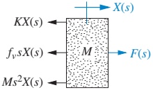
1‑DOF Translational: Impedance Picture

From the FBD, in the \(s\)‑domain each force is of the form

\[ F(s) = Z_M(s) X(s) \]

So in Figure 2.16(b):

Figure 2.16(b): Transformed FBD with impedances

We get directly:

\[ [Ms^{2}+f_{v}s+K]X(s) = F(s) \]

This is of the form

\[ [\text{Sum of impedances}] \cdot X(s) = [\text{Sum of applied forces}] \]

similar (but not strictly analogous) to a mesh equation.

Point out: this is purely algebra; no derivatives appear explicitly once we are in the \(s\)‑domain. This is the power of Laplace + impedance.

Degrees of Freedom (DOF)

Definition:

• A system’s number of degrees of freedom (DOF) = number of independent motions.
• A point of motion is independent if it can move while all other points are held still.

Consequences:

• Number of DOF = number of independent equations of motion needed.
• Motions are usually coupled (springs, dampers) but still count as separate DOF.

Analogy with circuits:

• In a 2‑loop circuit, two mesh currents: 2 equations.
• In a 2‑mass mechanical system, two independent displacements: 2 equations.

Tip

To solve:

1. Draw a free-body diagram for each DOF.
2. Write force balance (Newton’s law) for each.
3. Laplace transform the set of equations and solve for the desired transfer function.

Use a physical example: two masses connected by a spring on a frictionless surface. Each can move independently if the other is held fixed.

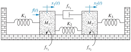
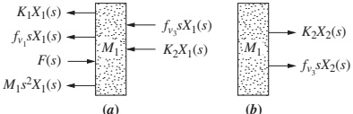
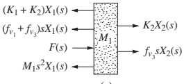
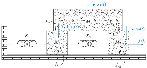
Example 2.17: Two-DOF Translational System

Problem:

Find transfer function \(G(s) = \dfrac{X_2(s)}{F(s)}\) for the system in Figure 2.17(a).

• Two masses \(M_1, M_2\)
• Springs \(K_1, K_2, K_3\)
• Dampers \(f_{v1}, f_{v2}, f_{v3}\)

DOF:

• \(x_1(t)\): motion of \(M_1\)
• \(x_2(t)\): motion of \(M_2\)

\(\Rightarrow\) 2 equations of motion needed.

Figure 2.17(a): 2‑DOF translational system

Figure 2.17(b): Block diagram

Tell students: This is like two “masses on a track” with couplings. Goal: show how superposition is used to systematically derive equations.

Example 2.17: Superposition for FBDs

To get forces on \(M_1\):

1. Move \(M_1\) to the right, hold \(M_2\) still → forces due to \(M_1\)’s own motion.
2. Hold \(M_1\) still, move \(M_2\) to the right → forces on \(M_1\) due to \(M_2\)’s motion.
3. Add the two sets of forces (superposition) → total forces on \(M_1\).

Figures 2.18(a–c) illustrate this:

Forces on M1 due to motions

All forces on M1

Similarly for \(M_2\) using Figures 2.19(a–c).

Key pedagogical point: Instead of guessing signs, we systematically build the FBD using superposition. This method becomes essential when systems get more complex.

Example 2.17: Equations of Motion (Laplace Form)

From the FBDs (Figures 2.18(c), 2.19(c)), we obtain in the Laplace domain:

\[ \big[M_{1}s^{2} + (f_{v_{1}}+f_{v_{3}})s + (K_{1}+K_{2})\big]X_{1}(s) - (f_{v_{3}}s+K_{2})X_{2}(s) = F(s) \]

\[ -(f_{v_{3}}s+K_{2})X_{1}(s) + \big[M_{2}s^{2} + (f_{v_{2}}+f_{v_{3}})s + (K_{2}+K_{3})\big]X_{2}(s) = 0 \]

We can write these in matrix form:

\[ \begin{bmatrix} Z_{11} & Z_{12} \\ Z_{21} & Z_{22} \end{bmatrix} \begin{bmatrix} X_1(s) \\ X_2(s) \end{bmatrix} = \begin{bmatrix} F(s) \\ 0 \end{bmatrix} \]

where

• \(Z_{11}\) = sum of impedances connected to \(x_1\)
• \(Z_{22}\) = sum of impedances connected to \(x_2\)
• \(Z_{12} = Z_{21} = -(f_{v_3}s + K_2)\) = negative sum of impedances between \(x_1\) and \(x_2\)

Emphasize the pattern:

• Diagonal entries: “self” impedances (mass + all elements to ground).
• Off-diagonals: negative of coupling impedances.

This is the mesh-equation structure they already know.

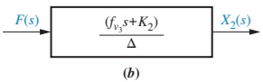
Example 2.17: Transfer Function

Solve the 2×2 system for \(X_2(s)/F(s)\):

\[ \frac{X_{2}(s)}{F(s)} = G(s) = \frac{(f_{v_{3}}s+K_{2})}{\Delta} \]

where

\[ \Delta=\left|\begin{array}{cc} M_{1}s^{2} + (f_{v_{1}}+f_{v_{3}})s + (K_{1}+K_{2}) & -(f_{v_{3}}s+K_{2})\\ -(f_{v_{3}}s+K_{2}) & M_{2}s^{2} + (f_{v_{2}}+f_{v_{3}})s + (K_{2}+K_{3}) \end{array}\right| \]

This is the determinant of the impedance matrix.

Note

Again, form is identical to a 2‑loop RLC circuit if we replace masses, springs, dampers with inductors, capacitors, resistors via the analogy.

If time permits, briefly show or mention how Cramer’s Rule leads to the numerator/denominator structure. You can also quickly discuss resonance and coupled modes for intuition, but keep the algebra the primary focus.

Example 2.18: 3‑DOF Translational — Equations by Inspection

Figure 2.20: 3‑DOF translational system

We have three masses → 3 DOF (\(x_1, x_2, x_3\)).

General patterns (mesh-style):

For \(M_1\):

\[ \big[\text{Sum of impedances connected to } x_1\big]X_{1}(s) - \big[\text{Impedances between } x_1 \text{ and } x_2\big] X_{2}(s) - \big[\text{Impedances between } x_1 \text{ and } x_3\big] X_{3}(s) = \big[\text{Sum of applied forces at } x_1\big] \]

Similar structures hold for \(x_2\) and \(x_3\).

This is an important conceptual leap: you can write equations by inspection from a network diagram, just like circuit mesh analysis, without individual FBDs.

Example 2.18: Final Equations

Using impedances (Table 2.4) and the pattern, we get:

For \(M_1\):

\[ [M_{1}s^{2} + (f_{v_{1}}+f_{v_{3}})s + (K_{1}+K_{2})]X_{1}(s) - K_{2}X_{2}(s) - f_{v_{3}}s X_{3}(s) = 0 \]

For \(M_2\):

\[ -K_{2}X_{1}(s) + [M_{2}s^{2} + (f_{v_{2}}+f_{v_{4}})s + K_{2}]X_{2}(s) - f_{v_{4}}sX_{3}(s) = F(s) \]

For \(M_3\):

\[ -f_{v_{3}}s X_{1}(s) - f_{v_{4}}s X_{2}(s) + [M_{3}s^{2}+(f_{v_{3}}+f_{v_{4}})s]X_{3}(s) = 0 \]

These are the equations of motion; we can solve for any \(X_i(s)\) or transfer function we need.

Point out that solving a 3×3 system is algebraically messier, but software (MATLAB, Python) handles it easily. The key skill is setting up the equations correctly.

Skill Assessment: Translational Practice (2.8)

Translational system for Skill-Assessment 2.8

Given system in Figure 2.21:

Task: Find \(G(s) = \dfrac{X_2(s)}{F(s)}\).

Answer provided:

\[ G(s) = \frac{3s + 1}{s(s^3 + 7s^2 + 5s + 1)} \]

Tip

Try to:

1. Identify DOF and define \(x_1(t)\), \(x_2(t)\), etc.
2. Write equations by inspection using mechanical impedances.
3. Solve the system to confirm the given \(G(s)\).

Complete solution is available on the book’s website.

Use this slide for in-class or homework reinforcement. Ask students to outline the steps even if they don’t fully compute the algebra in class.

Transition to Rotational Systems

We now move from translational to rotational systems.

The procedure is identical, except:

• Force \(f\) → Torque \(T\)
• Displacement \(x\) → Angular displacement \(\theta\)
• Velocity \(v\) → Angular velocity \(\omega\)
• Mass \(M\) → Moment of inertia \(J\)

Mechanical elements:

• Rotational spring (twist)
• Rotational damper (torsional friction)
• Inertia

Note

Everything we did for \(x(t)\) and \(f(t)\) now repeats for \(\theta(t)\) and \(T(t)\).

This is a good moment to connect to physical ECE systems: motors, gear trains, torsional shafts, disk drives.

Rotational Elements & Equations (Time Domain)

Table 2.5: Rotational analogs

Component	Torque–angular velocity	Torque–angular displacement
Spring	\(T(t) = K\displaystyle\int_{0}^{t}\omega(\tau)d\tau\)	\(T(t) = K\theta(t)\)
Viscous damper	\(T(t) = D\omega(t)\)	\(T(t) = D\dfrac{d\theta(t)}{dt}\)
Inertia	\(T(t) = J\dfrac{d\omega(t)}{dt}\)	\(T(t) = J\dfrac{d^{2}\theta(t)}{dt^{2}}\)

Units:

• \(T(t)\) – N·m
• \(\theta(t)\) – rad
• \(\omega(t)\) – rad/s
• \(K\) – N·m/rad
• \(D\) – N·m·s/rad
• \(J\) – kg·m²

Rotational impedance:

\[ Z_M(s) = \frac{T(s)}{\theta(s)} = \begin{cases} K & \text{(spring)} \\ Ds & \text{(damper)} \\ Js^2 & \text{(inertia)} \end{cases} \]

Point out how perfectly analogous this table is to Table 2.4. Students should be convinced that the same mathematical machinery applies.

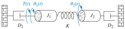
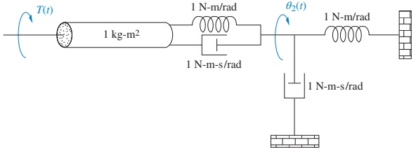
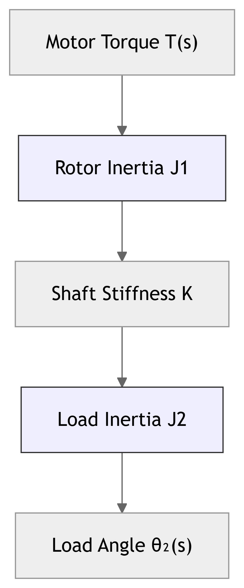
Rotational Example 2.19: Physical Setup

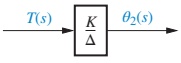
Problem:

Find \(G(s) = \dfrac{\theta_2(s)}{T(s)}\) for the system in Figure 2.22(a).

• A shaft undergoing torsion between two inertias \(J_1\) and \(J_2\).
• A torque input \(T(t)\) applied at the left.
• Output is angular displacement \(\theta_2\) at the right.

Modeling approximations:

• Shaft torsion modeled as a lumped spring of stiffness \(K\).
• Inertia on left = \(J_1\), on right = \(J_2\).
• Damping in shaft is negligible; local inertias have viscous damping \(D_1\), \(D_2\).

Figure 2.22(a–b): Physical system and schematic

Figure 2.22(a–b): Physical system and schematic

Figure 2.22(c): Block diagram

Mention that this models things like a motor connected to a load by a flexible shaft. The “springiness” of the shaft can introduce torsional oscillations.

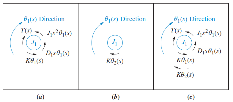
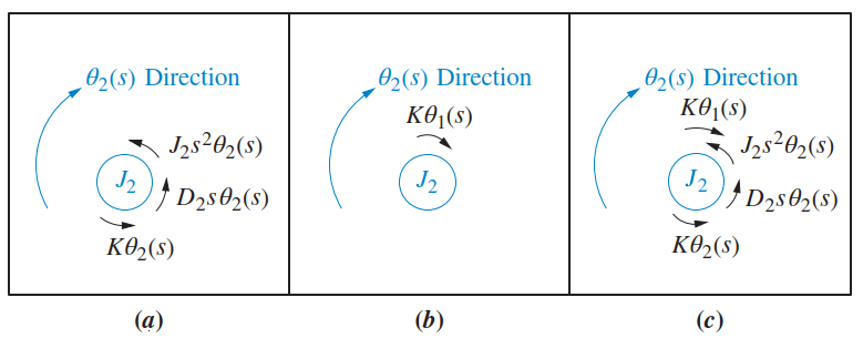
Example 2.19: Free-Body Diagrams by Superposition

We again use superposition:

For \(J_1\):

1. Rotate \(J_1\) with \(J_2\) fixed → torques due to \(J_1\)’s own motion (inertia, damping, spring twist).
2. Rotate \(J_2\) with \(J_1\) fixed → torques on \(J_1\) due to \(J_2\)’s motion (spring twist).
3. Add them → total torques on \(J_1\).

Torques on J1

Similarly for \(J_2\), using Figure 2.24.

Torques on J2

Explain the spring torque: \(K(\theta_1 - \theta_2)\). When you fix one angle and move the other, you get a torque proportional to their relative displacement.

Example 2.19: Equations of Motion (Laplace)

From the FBDs:

\[ (J_{1}s^{2}+D_{1}s+K)\theta_{1}(s)-K\theta_{2}(s)=T(s) \]

\[ -K\theta_{1}(s)+(J_{2}s^{2}+D_{2}s+K)\theta_{2}(s)=0 \]

Again, matrix form:

\[ \begin{bmatrix} J_{1}s^{2}+D_{1}s+K & -K\\ -K & J_{2}s^{2}+D_{2}s+K \end{bmatrix} \begin{bmatrix} \theta_1(s) \\ \theta_2(s) \end{bmatrix} = \begin{bmatrix} T(s) \\ 0 \end{bmatrix} \]

Solve for \(\theta_2(s)/T(s)\):

\[ \frac{\theta_{2}(s)}{T(s)}=\frac{K}{\Delta} \]

with

\[ \Delta=\left|\begin{array}{cc} J_{1}s^{2}+D_{1}s+K & -K\\ -K & J_{2}s^{2}+D_{2}s+K \end{array}\right| \]

Compare side-by-side with Example 2.17: same structure, just \(J,D,K,\theta\) instead of \(M,f_v,K,x\). This confirms that students can reuse translational intuition for rotational systems.

Example 2.19: MATLAB Support (TryIt 2.9)

In MATLAB with Symbolic Math Toolbox, the matrix equation can be solved symbolically:

syms s J1 D1 K T J2 D2 theta1 theta2

A = [J1*s^2 + D1*s + K,   -K;
     -K,                  J2*s^2 + D2*s + K];

B = [theta1; theta2];
C = [T; 0];

B = inv(A)*C;     % or B = A\C;
theta2 = B(2)
pretty(theta2)

This yields an expression matching

\[ \theta_2(s) = \frac{K}{\Delta} T(s) \]

Encourage students to use symbolic tools to check their algebra, but emphasize they should still be able to set up the equations themselves.

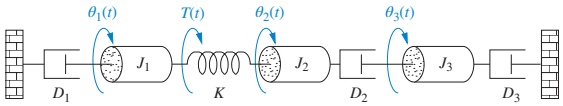
Example 2.20: 3‑DOF Rotational — Equations by Inspection

Figure 2.25: 3‑DOF rotational system

Angles: \(\theta_1, \theta_2, \theta_3\) → 3 DOF.

The generic pattern (mesh-style):

For \(\theta_1\):

• Sum of impedances connected to \(\theta_1\) times \(\theta_1(s)\)
• Minus each impedance between \(\theta_1\) and other DOF times the corresponding angle = Sum of applied torques at \(\theta_1\)

Same idea for \(\theta_2\) and \(\theta_3\).

This is the direct rotational analog of Example 2.18. Again, the main learning target is recognizing and applying the pattern.

Example 2.20: Final Equations

Applying the pattern:

\[ \begin{aligned} (J_{1}s^{2}+D_{1}s+K)\theta_{1}(s) &- K\theta_{2}(s) &- 0\theta_{3}(s) &= T(s) \\ -K\theta_{1}(s) &+ (J_{2}s^{2}+D_{2}s+K)\theta_{2}(s) &- D_{2}s\theta_{3}(s) &= 0\\ -0\theta_{1}(s) &- D_{2}s\theta_{2}(s) &+ (J_{3}s^{2}+D_{3}s+D_{2}s)\theta_{3}(s) &= 0 \end{aligned} \]

Again, we have a 3×3 linear system in \(\theta_1(s)\), \(\theta_2(s)\), \(\theta_3(s)\).

Note

These equations are ready to be solved for transfer functions like \(\theta_3(s)/T(s)\) or \(\theta_2(s)/T(s)\) using matrix methods.

Point out that cross-coupling appears in the off-diagonal terms: \(-K\) and \(-D_2 s\). Students should see how springs and dampers “connect” DOFs just like resistors connect nodes or meshes.

Skill Assessment: Rotational Practice (2.9)

Rotational system for Skill-Assessment 2.9

Problem: For the system in Figure 2.26, find:

\[ G(s) = \frac{\theta_2(s)}{T(s)} \]

Answer:

\[ G(s) = \frac{1}{2s^{2} + s + 1} \]

Tip

Check yourself:

1. Identify DOF and define \(\theta_1\), \(\theta_2\).
2. Write FBDs or use impedance inspection.
3. Derive equations of motion in Laplace domain.
4. Solve for \(\theta_2(s)/T(s)\) and compare with the given answer.

Again, encourage students to actually attempt the derivation before checking the textbook solution online.

Real-World ECE Applications

Where do these models show up?

• DC motor position control:
  • Motor rotor → inertia \(J\)
  • Load gear/shaft → spring \(K\) (torsional flexibility) + damping \(D\)
• Servo systems (antenna pointing, camera gimbals):
  • Rotational shafts with compliance and damping.
• Hard disk drives / tape drives:
  • Rotational platters and head actuators.
• Robotics joints:
  • Link flexibilities modeled with springs/dampers; joint inertia modeled as \(J\).

In each case, the controller design relies on an accurate transfer function.

Tie back to the earlier torsional example: the motor–load shaft system is mathematically the same as Example 2.19. Highlight that modeling flexibility (non-rigid connections) is often crucial to avoid oscillations and instability.

Summary / Key Points

1. Translational elements:

   • Spring: \(f(t)=Kx(t)\), \(Z_M=K\)
   • Damper: \(f(t)=f_v \dfrac{dx}{dt}\), \(Z_M=f_v s\)
   • Mass: \(f(t)=M \dfrac{d^{2}x}{dt^{2}}\), \(Z_M=Ms^2\)

2. Rotational elements:

   • Spring: \(T(t)=K\theta(t)\), \(Z_M=K\)
   • Damper: \(T(t)=D \dfrac{d\theta}{dt}\), \(Z_M=Ds\)
   • Inertia: \(T(t)=J \dfrac{d^{2}\theta}{dt^{2}}\), \(Z_M=Js^2\)

3. Mechanical impedance \(Z_M(s)=\dfrac{F(s)}{X(s)}\) or \(\dfrac{T(s)}{\theta(s)}\) allows circuit-like analysis.

4. Degrees of freedom (DOF) = number of independent motions = number of equations of motion.

5. Equations of motion for multi-DOF systems resemble mesh equations:

   • Diagonal: sum of impedances connected to a DOF.
   • Off-diagonal: negative of impedances between DOFs.

6. Transfer functions are obtained by solving the Laplace-domain linear system for output over input.

Encourage students to reflect: can they now look at a mechanical drawing and (a) identify DOF, (b) write Laplace-domain equations by inspection? That’s the main competency from this part of the course.

Formula Summary (Cheat Sheet)

Translational:

• Spring: \[ f(t)=Kx(t), \quad F(s)=KX(s), \quad Z_M = K \]
• Damper: \[ f(t)=f_{v}\frac{dx}{dt}, \quad F(s)=f_{v}sX(s), \quad Z_M = f_v s \]
• Mass: \[ f(t)=M\frac{d^{2}x}{dt^{2}}, \quad F(s)=Ms^{2}X(s), \quad Z_M = Ms^2 \]

Rotational:

• Spring: \[ T(t)=K\theta(t), \quad T(s)=K\theta(s), \quad Z_M = K \]
• Damper: \[ T(t)=D\frac{d\theta}{dt}, \quad T(s)=Ds\theta(s), \quad Z_M = Ds \]
• Inertia: \[ T(t)=J\frac{d^{2}\theta}{dt^{2}}, \quad T(s)=Js^{2}\theta(s), \quad Z_M = Js^2 \]

General transfer function pattern (1‑DOF):

• Translational: \(G(s)=\dfrac{X(s)}{F(s)} = \dfrac{1}{Ms^{2}+f_v s + K}\)
• Rotational: \(G(s)=\dfrac{\theta(s)}{T(s)} = \dfrac{1}{Js^{2}+Ds + K}\)

Suggest students copy this slide into their notes as a reference. They will use these formulas repeatedly in later chapters (time response, root locus, frequency response, controller design).

Next Steps

For practice before the next class:

1. Re-derive the answers for Skill-Assessment Exercises 2.8 and 2.9.
2. Try creating your own 2‑DOF mechanical system (translational or rotational), draw it, and write its equations of motion by inspection.
3. In the next lecture, we will extend these ideas to systems with electrical and mechanical parts together (mechatronic systems) and discuss how to cascade their transfer functions.

Wrap up by reinforcing continuity: next topic will integrate these mechanical models with electrical subsystems, completing the picture for many real ECE control problems.

Translational & Rotational Mechanical Systems – Interactive Addendum

Addendum Interactive Deck

How This Interactive Deck Works

This addendum lets you experiment with the ideas from Sections 2.5–2.6 directly in the browser.

You will:

• Tweak mass–spring–damper and rotational parameters and see how transfer functions and responses change.
• Use Pyodide (Python in WebAssembly) for live code execution.
• Use Observable JS (OJS) sliders + Pyodide + Plotly for reactive plots.

Tips:

• Change parameters and re‑run code blocks to see immediate effects.
• Focus on the connection between physical parameters (\(M, f_v, K, J, D\)) and the resulting transfer function / response.

1. Translational Mass–Spring–Damper: Build the Transfer Function

Use this interactive Python cell to compute the transfer function

\[ G(s) = \frac{X(s)}{F(s)} = \frac{1}{Ms^2 + f_v s + K} \]

for user‑chosen parameters.

Try:

• Set fv_val = 0.0 to see the undamped transfer function.
• Increase fv_val and observe how the denominator changes.

2. Translational System: Explore Pole Locations

The poles of \(G(s)\) are the roots of \(Ms^2 + f_v s + K = 0\).

Use this block to compute the poles for your chosen parameters.

Questions to think about:

• When are the poles real vs. complex?
• How does increasing damping \(f_v\) move the poles?

3. Reactive Plot: Translational Step Response vs. Parameters

Use the sliders to adjust \(M\), \(f_v\), and \(K\). A step response of the mass–spring–damper system will update automatically.

viewof M_tr = Inputs.range([0.2, 5], {step: 0.2, label: "Mass M (kg)", value: 1})
viewof fv_tr = Inputs.range([0, 10], {step: 0.5, label: "Damping f_v (N·s/m)", value: 2})
viewof K_tr = Inputs.range([0.5, 20], {step: 0.5, label: "Stiffness K (N/m)", value: 5})

Try:

• Set fv_tr = 0 and see the oscillatory behavior.
• Increase fv_tr and observe the motion become more damped.
• Change K_tr to see how the stiffness changes the oscillation frequency.

4. Visualizing Mechanical Impedance Magnitudes

Mechanical impedances in the \(s=j\omega\) domain:

• Mass: \(Z_M(j\omega) = M (j\omega)^2 = -M\omega^2\)
• Damper: \(Z_M(j\omega) = f_v (j\omega)\)
• Spring: \(Z_M(j\omega) = K\)

Use sliders to vary \(M\), \(f_v\), and \(K\), and see how the magnitude of each changes over frequency.

viewof M_imp = Inputs.range([0.2, 5], {step: 0.2, label: "Mass M for impedance", value: 1})
viewof fv_imp = Inputs.range([0, 10], {step: 0.5, label: "Damping f_v for impedance", value: 2})
viewof K_imp = Inputs.range([0.5, 20], {step: 0.5, label: "Stiffness K for impedance", value: 5})

Observe:

• At low frequency, which element dominates?
• At high frequency, which element dominates?
• How does increasing each parameter shift the curves?

5. 2‑DOF Translational System: Interactive Coefficients

Consider the 2‑DOF system from Example 2.17. We focus on the diagonal terms of the impedance matrix:

• \(Z_{11} = M_1 s^2 + (f_{v1}+f_{v3})s + (K_1 + K_2)\)
• \(Z_{22} = M_2 s^2 + (f_{v2}+f_{v3})s + (K_2 + K_3)\)

Use sliders to choose parameters and see how the coefficients of \(s^2\), \(s\), and constant terms change.

viewof M1_2dof = Inputs.range([0.5, 5], {step: 0.5, label: "M1 (kg)", value: 1})
viewof M2_2dof = Inputs.range([0.5, 5], {step: 0.5, label: "M2 (kg)", value: 2})

viewof fv1_2dof = Inputs.range([0, 10], {step: 0.5, label: "f_v1 (N·s/m)", value: 1})
viewof fv2_2dof = Inputs.range([0, 10], {step: 0.5, label: "f_v2 (N·s/m)", value: 1})
viewof fv3_2dof = Inputs.range([0, 10], {step: 0.5, label: "f_v3 (N·s/m)", value: 2})

viewof K1_2dof = Inputs.range([0, 20], {step: 1, label: "K1 (N/m)", value: 2})
viewof K2_2dof = Inputs.range([0, 20], {step: 1, label: "K2 (N/m)", value: 5})
viewof K3_2dof = Inputs.range([0, 20], {step: 1, label: "K3 (N/m)", value: 3})

Use this to see the mesh-like pattern:

• Diagonal terms: “self” impedances.
• Off-diagonal: negative of “between” impedances.

6. Rotational System: Build the Transfer Function

Now switch to rotational systems. For a 1‑DOF rotational system (spring–damper–inertia):

\[ G(s) = \frac{\theta(s)}{T(s)} = \frac{1}{Js^2 + D s + K} \]

Experiment with this interactive block.

Compare this form with the translational case. They are structurally identical, just with different physical units.

7. Rotational 2‑DOF (Example 2.19): Impedance Matrix Exploration

For Example 2.19, the equations are:

\[ (J_{1}s^{2}+D_{1}s+K)\theta_{1}(s)-K\theta_{2}(s)=T(s) \]

\[ -K\theta_{1}(s)+(J_{2}s^{2}+D_{2}s+K)\theta_{2}(s)=0 \]

Use sliders to explore the impedance matrix and its determinant \(\Delta\).

viewof J1_rot = Inputs.range([0.1, 5], {step: 0.1, label: "J1 (kg·m²)", value: 0.5})
viewof J2_rot = Inputs.range([0.1, 5], {step: 0.1, label: "J2 (kg·m²)", value: 1.0})

viewof D1_rot = Inputs.range([0, 5], {step: 0.2, label: "D1 (N·m·s/rad)", value: 0.5})
viewof D2_rot = Inputs.range([0, 5], {step: 0.2, label: "D2 (N·m·s/rad)", value: 0.5})

viewof K_rot = Inputs.range([0.5, 20], {step: 0.5, label: "K (N·m/rad)", value: 5})

Reflect:

• How does increasing \(K\) affect \(\Delta\) and \(G(s)\)?
• What happens if you increase \(D_1\) or \(D_2\)?

8. Rotational 1‑DOF: Reactive Step Response

Use sliders to adjust \(J\), \(D\), and \(K\) and see the step response in angle \(\theta(t)\).

viewof J_step = Inputs.range([0.1, 5], {step: 0.1, label: "J (kg·m²)", value: 1})
viewof D_step = Inputs.range([0, 5], {step: 0.1, label: "D (N·m·s/rad)", value: 0.5})
viewof K_step = Inputs.range([0.5, 20], {step: 0.5, label: "K (N·m/rad)", value: 3})

Explore:

• \(D = 0\) → purely oscillatory response.
• Larger \(D\) → more damping.
• Larger \(K\) → higher natural frequency.

9. Compare Translational vs Rotational Models Side-by-Side

Use this cell to print both transfer functions side-by-side for your chosen parameters.

Notice the pattern:

• Same mathematical structure, different physical meanings.
• This is why mechanical systems can be treated like RLC networks once we define appropriate analogies and impedances.

10. Your Turn: Design a Simple 2‑DOF System

Use this empty template to quickly prototype your own 2‑DOF translational system equations in Python.

Next challenge (outside this block):

• Assume input force \(F(s)\) acts at \(x_1\), write the right‑hand side vector, and solve for \(X_2(s)/F(s)\).

Wrap-Up: What You Should Take Away

Using these interactive blocks, you have:

• Manipulated mass–spring–damper and rotational system parameters and seen their impact on transfer functions and time responses.
• Observed how mechanical impedance shapes frequency response.
• Seen how multi‑DOF systems lead to mesh-like impedance matrices, just like in circuits.
• Practiced using symbolic and numerical tools (via Pyodide) to reinforce the theory from Sections 2.5–2.6.

Use this deck as a sandbox: modify code, change parameters, and relate every change you see back to the underlying physics + Laplace-domain algebra.