Modeling in the Frequency Domain

Sistem Kendali 2.1

Imron Rosyadi

Learning Objectives

By the end of this session, you will be able to:

• Explain why control engineers prefer transfer functions over raw differential equations.
• Recall and use key Laplace transform pairs and theorems.
• Perform partial‑fraction expansion for real, repeated, and complex roots.
• Use Laplace transforms to solve linear differential equations with zero initial conditions.
• Define and compute a transfer function from a given differential equation.
• Relate simple transfer functions to time‑domain responses (step, ramp) relevant to ECE systems.

This slide sets expectations. Emphasize the “why” (motivation) first: modeling in the frequency domain lets us separate input/system/output and use algebra instead of calculus. Then connect each objective to a concrete action they’ll perform in examples or interactive blocks.

From Differential Equations to Block Diagrams

• Many physical systems → differential equations (DEs) relating input and output.
• But DEs:
  • Mix input, output, and parameters everywhere.
  • Are hard to interconnect for multi‑block systems.
• We want:
  • A clean separation: input, system, output.
  • Simple rules for connecting subsystems in cascade, feedback, etc.

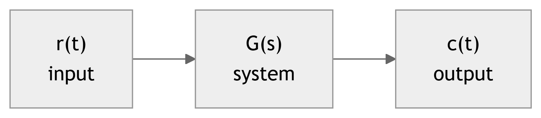
Single block:

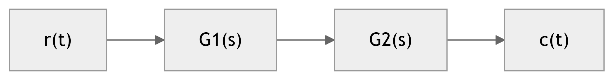
Cascaded blocks:

Relate to a concrete example from Chapter 1: a position control system with motor + gear + load. In DE form, parameters for each physical part are intermingled. In block form, each is a block with its own transfer function. Point out that for cascaded blocks, the overall transfer function is simply the product of individual transfer functions G1(s)G2(s), which is far easier than combining DEs directly.

Why Frequency‑Domain Modeling?

• Laplace transform:
  • Handles exponentials and sinusoids.
  • Turns \(d/dt\) into multiplication by \(s\).
• This leads to transfer functions: algebraic ratios in \(s\) that:
  • Model circuits, motors, sensors, amplifiers.
  • Are easy to connect and analyze.

Tip

Think: time domain = “oscilloscope view”. Laplace/frequency domain = “algebra and plots” view for design.

Make explicit analogy: phasors are to sinusoidal steady state as Laplace transforms are to full transient + steady state. Remind them that \(s = \sigma + j\omega\); phasors correspond to the special case \(\sigma = 0\). This helps ECE students connect current knowledge to Laplace and transfer functions.

Laplace Transform: Definition

We define the (unilateral) Laplace transform as

\[ \mathcal{L}[f(t)] = F(s) = \int_{0^-}^{\infty} f(t) e^{-st}\, dt,\quad s=\sigma + j\omega \]

• \(f(t)\): time‑domain signal (usually \(t\ge 0\) in control).
• \(F(s)\): Laplace‑domain representation.
• Lower limit \(0^-\) means we can handle discontinuities at \(t=0\), including impulses.

Inverse Laplace transform:

\[ \mathcal{L}^{-1}[F(s)] = \frac{1}{2\pi j} \int_{\sigma - j\infty}^{\sigma + j\infty} F(s)e^{st} ds = f(t) u(t) \]

• \(u(t)\): unit step, forcing causality (zero for \(t<0\)).

Stress that in control we almost always use the unilateral transform (starting at 0^-), because we care about system response after an input is applied. Emphasize that the inverse integral is not something they will compute by hand; instead, they’ll use tables and partial fractions.

Key Laplace Transform Pairs (Table 2.1 Excerpts)

Time domain \(f(t)\)

1. \(\delta(t)\)
2. \(u(t)\)
3. \(t u(t)\)
4. \(t^{n}u(t)\)
5. \(e^{-a t} u(t)\)
6. \(\sin \omega t \, u(t)\)
7. \(\cos \omega t \, u(t)\)

Laplace domain \(F(s)\)

1. \(1\)
2. \(\dfrac{1}{s}\)
3. \(\dfrac{1}{s^{2}}\)
4. \(\dfrac{n!}{s^{n+1}}\)
5. \(\dfrac{1}{s + a}\)
6. \(\dfrac{\omega}{s^{2} + \omega^{2}}\)
7. \(\dfrac{s}{s^{2} + \omega^{2}}\)

Important

These seven pairs cover most standard test signals in control: impulse, step, ramp, exponentials, and sinusoids. You should be able to recognize and use them without a table over time.

Encourage students to memorize at least the impulse, step, ramp, exponential, and sin/cos pairs. Point out that many more complicated transforms can be built using these plus the theorems (shift, scaling, differentiation).

Interactive Check: Compute a Simple Laplace Transform

Use the definition to compute the Laplace transform of \(f(t) = Ae^{-at}u(t)\).

Walk through the steps from the output: they should see A/(s+a). Connect this back to Item 5 in Table 2.1 and to Example 2.1. Emphasize that we can always fall back to the integral definition when in doubt.

Example 2.1 – Laplace Transform of \(A e^{-a t} u(t)\)

We want \(\mathcal{L}[f(t)]\) for \(f(t) = A e^{-a t} u(t)\).

Since there is no impulse at \(t=0\), we can start at 0:

\[ \begin{aligned} F(s) &= \int_{0}^{\infty} A e^{-a t} e^{-s t} dt \\ &= A \int_{0}^{\infty} e^{-(s + a)t} dt \\ &= -\frac{A}{s+a} e^{-(s+a)t} \bigg|_{0}^{\infty} \\ &= \frac{A}{s+a} \end{aligned} \]

So

\[ \mathcal{L}[A e^{-a t} u(t)] = \frac{A}{s + a} \]

Show the convergence reasoning: the exponential term goes to zero as \(t \to \infty\) if \(\text{Re}(s+a) > 0\). Also highlight that \(A\) just factors out (linearity).

Laplace Transform Theorems

Linearity

• \(\mathcal{L}[k f(t)] = k F(s)\)
• \(\mathcal{L}[f_1(t) + f_2(t)] = F_1(s) + F_2(s)\)

Frequency shift

• \(\mathcal{L}[e^{-a t} f(t)] = F(s + a)\)

Differentiation in time

• \(\mathcal{L}\left[\dfrac{df}{dt}\right] = sF(s) - f(0^-)\)

Integration in time

• \(\mathcal{L}\left[\int_0^t f(\tau)\, d\tau \right] = \dfrac{F(s)}{s}\)

Value theorems:

• Final value: \(f(\infty) = \displaystyle\lim_{s\to 0} s F(s)\) (under stability conditions).
• Initial value: \(f(0^+) = \displaystyle\lim_{s\to\infty} s F(s)\) (under continuity conditions).

Warning

Value theorems have conditions:

• Final value only if all poles of \(sF(s)\) have negative real parts or at most one at the origin.
• Initial value only if \(f(t)\) has no impulses at \(t=0\).

Explain that these theorems are tools to avoid doing full inverses. In control design we often care about steady‑state error → final value theorem is heavily used. Give a quick mental example: step response of 1/(s+2) has \(C(s)=1/(s(s+2))\), so \(c(\infty) = \lim_{s→0} s /(s(s+2)) = 1/2\), matching the time‑domain expression.

Inverse Laplace via Tables & Theorems – Example 2.2

Given:

\[ F_1(s) = \frac{1}{(s+3)^2} \]

We know from Table 2.1:

• \(\mathcal{L}[t u(t)] = \dfrac{1}{s^2}\).

Use the frequency shift theorem:

• If \(\mathcal{L}[t] = \dfrac{1}{s^2}\), then \(\mathcal{L}[e^{-a t} t] = \dfrac{1}{(s + a)^2}\).

So with \(a = 3\):

\[ \mathcal{L}^{-1}\left[\frac{1}{(s+3)^2}\right] = e^{-3t} t u(t) \]

Ask students what \(f(t)\) would be if the denominator was \((s+3)^3\) to see if they infer \(t^2 e^{-3t}/2!\). Reinforce the pattern \(t^n u(t) \leftrightarrow n! / s^{n+1}\) and its shifted version.

Why Partial‑Fraction Expansion?

• Many \(F(s)\) arise as ratios of polynomials:

  \[ F(s) = \frac{N(s)}{D(s)},\quad \deg N < \deg D \]

• Usually not in table form directly.

• Strategy:

  1. Factor \(D(s)\) into simple factors.
  2. Express \(F(s)\) as a sum of simple terms.
  3. Use the table on each term.

Note

If \(\deg N \ge \deg D\), perform polynomial long division first to get polynomial + proper fraction (numerator degree < denominator degree).

Connect with circuits: when finding time response of an RLC network, the natural response terms come from the poles (roots of the denominator) and are exponentials or damped sinusoids. Partial fractions is how we expose these modes.

Example: Need for Long Division

Given

\[ F_1(s) = \frac{s^3 + 2s^2 + 6s + 7}{s^2 + s + 5} \]

Perform polynomial division:

\[ F_1(s) = s + 1 + \frac{2}{s^2 + s + 5} \]

Then inverse Laplace:

\[ f_1(t) = \frac{d\delta(t)}{dt} + \delta(t) + \mathcal{L}^{-1}\left[\frac{2}{s^2 + s + 5}\right] \]

• The polynomial part (\(s + 1\)) represents impulses and derivatives at \(t=0\).
• The proper fraction is where the physical transient lies.

Don’t dwell on the impulse terms for now; just point out: polynomial terms in \(s\) → combinations of \(\delta(t)\) and its derivatives. Our main interest in control is typically the proper fraction part (for \(t>0\) responses).

Case 1: Real, Distinct Poles

Example:

\[ F(s) = \frac{2}{(s+1)(s+2)} \]

Assume

\[ F(s) = \frac{K_1}{s+1} + \frac{K_2}{s+2} \]

Solve residues:

• Multiply by \((s+1)\) and set \(s=-1\) → \(K_1 = \dfrac{2}{-1+2} = 2\).
• Multiply by \((s+2)\) and set \(s=-2\) → \(K_2 = \dfrac{2}{-2+1} = -2\).

Case 1: Real, Distinct Poles

So

\[ F(s) = \frac{2}{s+1} - \frac{2}{s+2} \]

Inverse Laplace:

\[ f(t) = 2 e^{-t} - 2 e^{-2t} \]

Tip

For distinct real poles at \(-p_1, -p_2, ..., -p_n\):

\[ F(s) = \sum_{i=1}^n \frac{K_i}{s + p_i},\quad K_i = (s + p_i) F(s)\big|_{s = -p_i} \]

Stress the “cover‑up” trick for simple real poles: multiply by the factor, then substitute the corresponding root. Mention that the exponents in time domain correspond to pole locations (modes of the system).

Example 2.3 – DE Solution via Laplace (Setup)

Given system:

\[ \frac{d^2 y}{dt^2} + 12 \frac{dy}{dt} + 32 y = 32 u(t),\quad y(0^-) = 0,\ \dot{y}(0^-) = 0 \]

1. Take Laplace of each term using differentiation theorems and \(u(t) \leftrightarrow 1/s\):

\[ s^2 Y(s) + 12 s Y(s) + 32 Y(s) = \frac{32}{s} \]

2. Solve for \(Y(s)\):

\[ Y(s) = \frac{32}{s(s^2 + 12s + 32)} = \frac{32}{s (s+4)(s+8)} \]

Now we just need partial fractions.

Ask students to verify the factorization \((s^2+12s+32)=(s+4)(s+8)\). Note what the poles are: 0, −4, −8. This already hints at a step response with two decaying exponentials and a constant term.

Example 2.3 – Partial Fractions and Solution

Assume

\[ Y(s) = \frac{K_1}{s} + \frac{K_2}{s+4} + \frac{K_3}{s+8} \]

Use cover‑up method:

• \(K_1 = \dfrac{32}{(s+4)(s+8)}\bigg|_{s=0} = 1\)
• \(K_2 = \dfrac{32}{s(s+8)}\bigg|_{s=-4} = -2\)
• \(K_3 = \dfrac{32}{s(s+4)}\bigg|_{s=-8} = 1\)

Example 2.3 – Partial Fractions and Solution

So

\[ Y(s) = \frac{1}{s} - \frac{2}{s+4} + \frac{1}{s+8} \]

Inverse Laplace:

\[ y(t) = 1 - 2 e^{-4t} + e^{-8t} \]

Note

We often drop the explicit \(u(t)\) factor in notation, assuming causal systems with inputs applied at \(t=0\).

Interpret the result physically: final value is 1 (matches right‑hand side 32 with static gain 1). Two decaying exponentials represent system dynamics with time constants 1/4 and 1/8 s. You can also quickly check final value via \(\lim_{s\to0} sY(s)\).

Interactive Practice: Partial Fractions in Python

Try a partial‑fraction expansion of

\[ F(s) = \frac{2}{(s+1)(s+2)} \]

Modify the expression in the code cell to experiment with other denominators.

After running, discuss the output: Sympy should give 2/(s+1) - 2/(s+2). Encourage students to try a denominator with a repeated pole or quadratic term to observe how the structure of the result changes.

Case 2: Real, Repeated Poles

Example:

\[ F(s) = \frac{2}{(s+1)(s+2)^2} \]

We write:

\[ F(s) = \frac{K_1}{s+1} + \frac{K_2}{(s+2)^2} + \frac{K_3}{s+2} \]

Case 2: Real, Repeated Poles

Procedure:

1. \(K_1\) via cover‑up (still simple pole):
   • Multiply by \((s+1)\) and set \(s=-1\): \(K_1 = 2\).
2. \(K_2\) isolate by multiplying by \((s+2)^2\) and setting \(s=-2\):
   • \(K_2 = -2\).
3. For \(K_3\) (other term in repeated root):
   • Differentiate the expression where \((s+2)^2 F(s)\) is isolated, then set \(s=-2\) to solve for \(K_3\): \(K_3 = -2\).

So

\[ f(t) = 2 e^{-t} - 2 t e^{-2t} - 2 e^{-2t} \]

Tip

For a repeated pole at \(s = -p\) of multiplicity \(r\), the expansion is

\[ \sum_{i=1}^r \frac{K_i}{(s+p)^i} \]

Corresponding time terms are of the form \(t^{i-1} e^{-p t}\).

Highlight that repeated poles lead to polynomial factors in time (e.g., \(t e^{-2t}\)), which correspond to non‑distinct system modes, such as critically damped or higher‑order repeated behavior.

Case 3: Complex or Imaginary Poles

Example:

\[ F(s) = \frac{3}{s(s^2 + 2s + 5)} \]

We use

\[ F(s) = \frac{K_1}{s} + \frac{K_2 s + K_3}{s^2 + 2s + 5} \]

1. \(K_1 = \dfrac{3}{5}\).
2. Multiply both sides by \(s(s^2+2s+5)\) and equate coefficients to find \(K_2\), \(K_3\).
   • Result: \(K_2 = -\dfrac{3}{5}\), \(K_3 = -\dfrac{6}{5}\).

Case 3: Complex or Imaginary Poles

So

\[ F(s) = \frac{3/5}{s} - \frac{3}{5}\frac{s+2}{s^2 + 2s + 5} \]

Complete the square:

\[ s^2 + 2s + 5 = (s + 1)^2 + 2^2 \]

Rewrite:

\[ F(s) = \frac{3/5}{s} - \frac{3}{5} \frac{(s+1) + 1}{(s+1)^2 + 4} \]

Match with

\[ \mathcal{L}[A e^{-a t}\cos\omega t + B e^{-a t}\sin\omega t] = \frac{A(s+a) + B\omega}{(s+a)^2 + \omega^2} \]

Yield

\[ f(t) = \frac{3}{5} - \frac{3}{5} e^{-t}\left(\cos 2t + \frac{1}{2} \sin 2t\right) \]

Or equivalently

\[ f(t) = 0.6 - 0.671 e^{-t} \cos(2t - \phi), \quad \phi \approx 26.57^\circ \]

Note

Complex poles → damped sinusoidal modes (oscillations that decay over time). This is crucial for understanding underdamped systems (e.g., RLC circuits, motor torque responses).

Emphasize geometric interpretation: complex poles at \(-1 \pm j2\) have real part −1 (decay rate) and imaginary part 2 (oscillation frequency). Students will see these again in second‑order system analysis.

Alternate Complex‑Residue Method (Outline)

We can also expand

\[ \frac{3}{s(s^2+2s+5)} = \frac{3}{s(s+1+j2)(s+1-j2)} \]

as

\[ F(s) = \frac{K_1}{s} + \frac{K_2}{s+1+j2} + \frac{K_3}{s+1-j2} \]

• \(K_2\) and \(K_3\) are complex conjugates.

• After inverse Laplace, exponentials with \(e^{\pm j2t}\) combine via

  \[ \cos\theta = \frac{e^{j\theta}+e^{-j\theta}}{2},\quad \sin\theta = \frac{e^{j\theta}-e^{-j\theta}}{2j} \]

to the same real expression as before.

This method is more algebraically heavy and conceptually advanced. Mention that computational tools (MATLAB, Python) often give complex residues, but the physical time‑domain solution is real, obtained by combining conjugate pairs.

Interactive Slider: Visualizing a Damped Sinusoid

viewof a = Inputs.range([0, 2], {step: 0.1, value: 1, label: "decay rate a"})
viewof w = Inputs.range([0, 5], {step: 0.5, value: 2, label: "frequency ω"})

Invite students to move sliders and observe how increasing a speeds up decay, while changing ω changes oscillation frequency. Connect back to the example with poles at −1 ± j2, so a=1, ω=2. This is a bridge to second‑order system classification.

Skill‑Assessment: Quick Laplace Transform

Exercise 2.1: Find \(\mathcal{L}[f(t)]\) for \(f(t) = t e^{-5t} u(t)\).

Using Table 2.1 and frequency shift:

• \(t u(t) \leftrightarrow 1/s^2\).
• Multiply by \(e^{-5t}\) → shift \(s \to s+5\):

\[ \mathcal{L}[t e^{-5t} u(t)] = \frac{1}{(s + 5)^2} \]

Encourage students to do this mentally: identify base transform, then apply shift. Ask them what the ROC (region of convergence) condition is: Re(s) > −5.

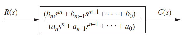
Laplace Transform → Transfer Function

We now connect Laplace transforms to transfer functions.

Start from a general LTI differential equation:

\[ a_n \frac{d^n c}{dt^n} + a_{n-1} \frac{d^{n-1} c}{dt^{n-1}} + \cdots + a_0 c(t) = b_m \frac{d^m r}{dt^m} + \cdots + b_0 r(t) \]

Take Laplace transforms (with zero initial conditions):

\[ (a_n s^n + a_{n-1} s^{n-1} + \cdots + a_0) C(s) = (b_m s^m + b_{m-1} s^{m-1} + \cdots + b_0) R(s) \]

Form the ratio

\[ \frac{C(s)}{R(s)} = G(s) = \frac{b_m s^m + b_{m-1} s^{m-1} + \cdots + b_0} {a_n s^n + a_{n-1} s^{n-1} + \cdots + a_0} \]

This \(G(s)\) is the transfer function:

• Describes the system alone (zero initial conditions).
• Input/output relationship: \(C(s) = G(s) R(s)\).

Important

The denominator of \(G(s)\) is the characteristic polynomial. Its roots → poles → fundamental dynamics (stability, oscillation, speed).

Highlight that initial conditions enter the Laplace transform as extra terms, but for the transfer function definition we set them to zero to isolate pure system behavior. Make sure they see that this is why the ratio is independent of particular initial conditions.

Transfer Function Block Representation

Block diagram of a transfer function

• Input: \(R(s)\) (Laplace transform of \(r(t)\)).
• Output: \(C(s)\) (Laplace transform of \(c(t)\)).
• Block: \(G(s)\) (system).
• Relationship: \(C(s) = G(s) R(s)\).

Relate this picture back to Figure 2.1 and to state the main advantage: we can now treat cascades, feedback loops, and other interconnections via algebra on these \(G(s)\) blocks rather than combining differential equations directly.

Example 2.4 – Transfer Function from DE

Given DE:

\[ \frac{dc}{dt} + 2c(t) = r(t) \]

1. Laplace transform with zero initial conditions:

\[ s C(s) + 2 C(s) = R(s) \]

2. Solve for \(C(s)/R(s)\):

\[ G(s) = \frac{C(s)}{R(s)} = \frac{1}{s + 2} \]

So the system is a first‑order low‑pass with pole at \(s = -2\).

Point out physical analogies: this could represent an RC or RL circuit, or a simple thermal or mechanical first‑order system. The time constant is 1/2 s. Ask: what’s the DC gain? (1/2 if we consider step input; actually the transfer function’s DC gain is 1/2 only if the input is a step – help them separate system gain vs full step response).

Example 2.5 – Step Response from \(G(s)\)

We use \(G(s) = 1/(s+2)\) and input \(r(t) = u(t)\).

1. Laplace of input: \(R(s) = 1/s\).
2. Output transform:

\[ C(s) = G(s) R(s) = \frac{1}{s(s+2)} \]

3. Partial fractions:

\[ C(s) = \frac{1/2}{s} - \frac{1/2}{s+2} \]

Example 2.5 – Step Response from \(G(s)\)

4. Inverse Laplace:

\[ c(t) = \frac{1}{2} - \frac{1}{2} e^{-2t} \]

Interpretation:

• Starts at 0, asymptotically approaches 0.5.
• Time constant: 0.5 s → at \(t = 0.5\) s, ~63% of the way to 0.5.

Tip

You can check final value via final value theorem:

\[ c(\infty) = \lim_{s\to0} s \cdot C(s) = \lim_{s\to0} \frac{s}{s(s+2)} = \frac{1}{2} \]

If time permits, sketch or quickly plot the response. Emphasize that this procedure (transfer function + Laplace of input + partial fractions) is the standard pipeline for computing time responses.

Interactive Plot: First‑Order Step Response

viewof a1 = Inputs.range([0.1, 5], {step: 0.1, value: 2, label: "Pole at s = -a"})

Explain that for G(s)=a/(s+a), DC gain is 1. Students can see how moving the pole (changing a) affects how fast the system responds: larger a → faster exponential decay. Link pole position in s‑plane to speed of response, a central theme in control.

Additional Skill‑Assessment Examples

• Exercise 2.3: From DE

  \[ \frac{d^3 c}{dt^3} + 3\frac{d^2 c}{dt^2} + 7\frac{dc}{dt} + 5c = \frac{d^2 r}{dt^2} + 4\frac{dr}{dt} + 3r \]

  Transfer function:

  \[ G(s) = \frac{s^2 + 4s + 3}{s^3 + 3s^2 + 7s + 5} \]

• Exercise 2.4: From \(G(s)\) back to DE:

  \[ G(s) = \frac{2s + 1}{s^2 + 6s + 2} \]

  multiply both sides by denominator and inverse Laplace to get

  \[ \frac{d^2 c}{dt^2} + 6\frac{dc}{dt} + 2c = 2\frac{dr}{dt} + r \]

Additional Skill‑Assessment Examples

• Exercise 2.5: Ramp response from \(G(s) = \dfrac{s}{(s+4)(s+8)}\)

  • Ramp input: \(r(t) = t u(t) \Rightarrow R(s) = 1/s^2\).
  • Then \(C(s) = G(s)R(s)\), do partial fractions, invert.

You don’t need to derive these fully in class, but use them to illustrate both directions: DE → G(s) and G(s) → DE, and also different inputs (step, ramp). Emphasize ramp as modeling linearly increasing commands, like a linearly increasing set‑point voltage or speed reference.

Real‑World ECE Application Examples

1. RC low‑pass filter

• Circuit: resistor R in series, capacitor C to ground.

• Input: \(v_{in}(t)\), output: \(v_{out}(t)\) across C.

• DE:

  \[ RC \frac{dv_{out}}{dt} + v_{out} = v_{in} \]

• Transfer function:

  \[ G(s) = \frac{V_{out}(s)}{V_{in}(s)} = \frac{1}{RC s + 1} \]

2. DC motor speed control (simplified)

• Input: armature voltage \(V_a(t)\).

• Output: angular speed \(\omega(t)\).

• Linearized model often:

  \[ J \frac{d\omega}{dt} + B \omega = K_t i_a,\quad L \frac{di_a}{dt} + R i_a + K_e \omega = V_a \]

• Combine and Laplace to get \(G(s) = \Omega(s)/V_a(s)\): typically a second‑order transfer function.

Use the RC filter as a simple first‑order transfer function example where students can easily map component values to pole location. For the DC motor, you don’t need to derive the full \(G(s)\) in detail now; just show that the same Laplace and DE tools extend directly to more complex systems in controls.

Summary / Key Points

• Laplace transform converts time‑domain functions and differential equations into algebraic expressions in \(s\).
• Laplace pairs and theorems (linearity, shift, differentiation, integration, value theorems) are essential tools.
• Partial‑fraction expansion is the main technique to invert rational \(F(s)\):
  • Case 1: real distinct poles → sums of exponentials.
  • Case 2: repeated poles → exponentials times polynomials in \(t\).
  • Case 3: complex poles → exponentially damped sinusoids.
• A transfer function \(G(s) = C(s)/R(s)\) (zero initial conditions) cleanly separates input, system, and output and corresponds to block diagrams.
• From a DE ↔︎ transfer function:
  • DE → Laplace → algebra → \(C(s)/R(s) = G(s)\).
  • \(G(s)\) + input Laplace → \(C(s)\) → partial fractions → \(c(t)\).

Reinforce that everything in later Chapters 2–6 (root locus, Bode plots, steady‑state error) will assume comfort with Laplace transforms and transfer functions. Encourage students to practice going back and forth between differential equations, transfer functions, and time‑domain responses.

Formulas Summary

Laplace transform definition:

\[ \mathcal{L}[f(t)] = F(s) = \int_{0^-}^{\infty} f(t) e^{-s t}\, dt \]

Inverse Laplace:

\[ \mathcal{L}^{-1}[F(s)] = \frac{1}{2\pi j} \int_{\sigma - j\infty}^{\sigma + j\infty} F(s)e^{st}\, ds = f(t)u(t) \]

Formulas Summary

Selected transform pairs:

• \(\delta(t) \leftrightarrow 1\)
• \(u(t) \leftrightarrow \dfrac{1}{s}\)
• \(t^n u(t) \leftrightarrow \dfrac{n!}{s^{n+1}}\)
• \(e^{-at} u(t) \leftrightarrow \dfrac{1}{s+a}\)
• \(\sin \omega t\, u(t) \leftrightarrow \dfrac{\omega}{s^2 + \omega^2}\)
• \(\cos \omega t\, u(t) \leftrightarrow \dfrac{s}{s^2 + \omega^2}\)

Formulas Summary

Key theorems:

• Linearity: \(\mathcal{L}[k f(t)] = kF(s)\), \(\mathcal{L}[f_1+f_2] = F_1+F_2\).
• Frequency shift: \(\mathcal{L}[e^{-at} f(t)] = F(s + a)\).
• Differentiation: \(\mathcal{L}\left[\dfrac{df}{dt}\right] = sF(s) - f(0^-)\).
• Integration: \(\mathcal{L}\left[\int_0^{t} f(\tau)d\tau\right] = \dfrac{F(s)}{s}\).
• Final value: \(f(\infty) = \lim_{s\to 0} sF(s)\) (under stability conditions).
• Initial value: \(f(0^+) = \lim_{s\to \infty} sF(s)\) (if no impulses at 0).

Transfer function (zero initial conditions):

• From DE:

  \[ \frac{C(s)}{R(s)} = G(s) = \frac{b_m s^m + \cdots + b_0} {a_n s^n + \cdots + a_0} \]

• Input–output relation:

  \[ C(s) = G(s) R(s) \]

Leave this as a concise reference slide. Suggest students copy or print it as a quick cheat‑sheet for homework and future lectures.