Introduction to Control Systems

Sistem Kendali 1

Imron Rosyadi

Learning Objectives

After this session, you will be able to:

• Define a control system and recognize common ECE applications.
• Distinguish open-loop and closed-loop (feedback) systems.
• Explain transient response, steady-state error, and stability qualitatively.
• Describe the main steps of the control system design process.
• Appreciate the role of computer-aided tools (e.g., MATLAB) in control design.
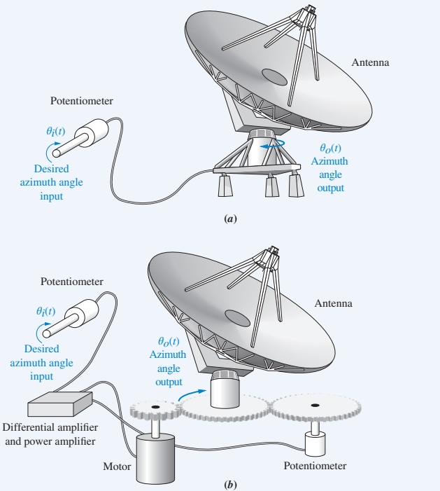
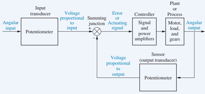
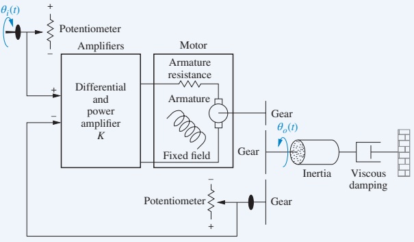
• Interpret the antenna-azimuth case study as a canonical position control problem.

Clarify that today’s focus is conceptual, with minimal equations. These objectives line up with Sections 1.1–1.7 of the text and the antenna case study. Point out that understanding this “big picture” will make the math in later chapters much more intuitive.

Big Picture: What Is a Control System?

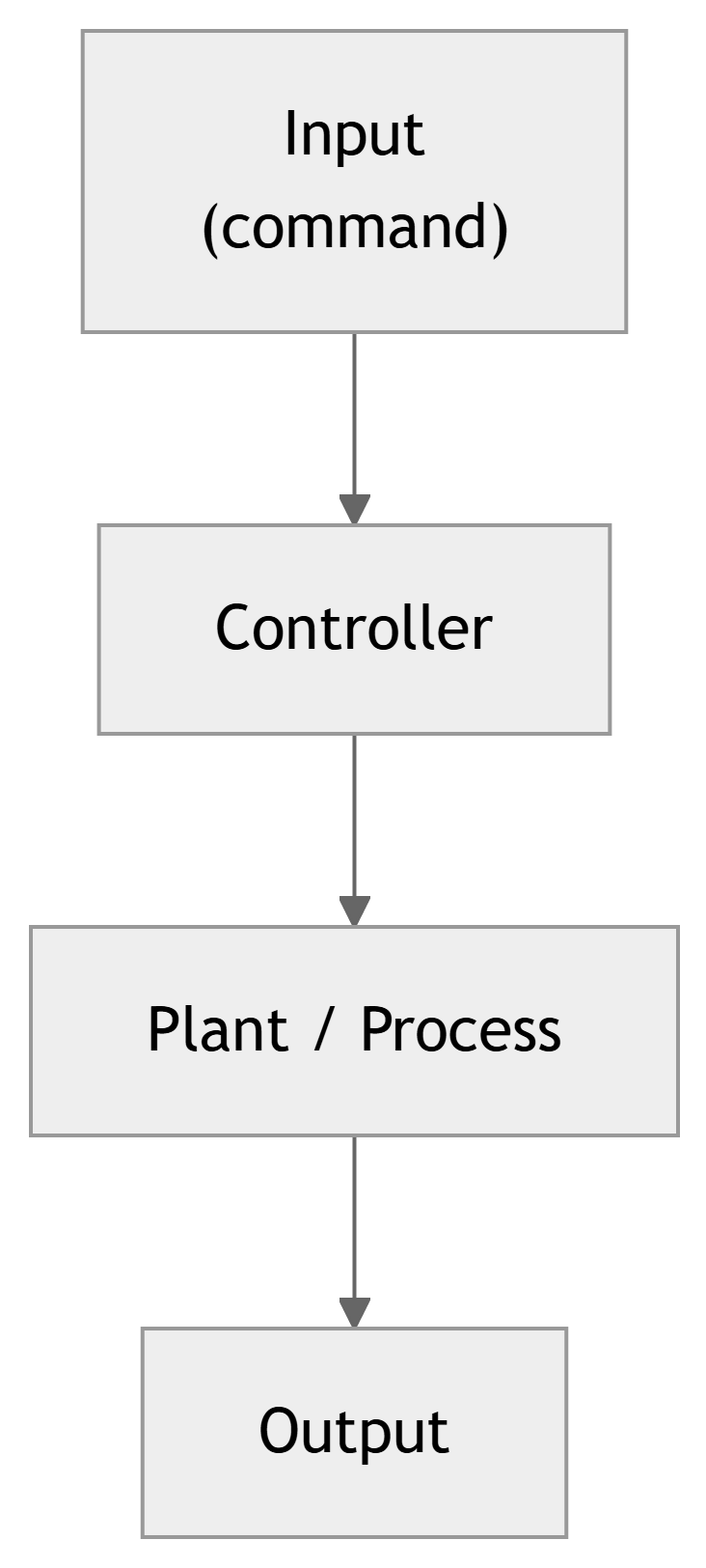
A control system is:

A collection of subsystems and processes (the plant) assembled to produce a desired output, with desired performance, in response to a specified input.

Key ingredients:

• Input (command / reference) – what we want.
• Plant / process – the physical system we influence.
• Output – what actually happens.
• Controller – logic that decides how to drive the plant.
• Optionally: feedback that measures the output.

Relate to something they know: - Audio volume knob → amplifier → speaker → sound level. - Temperature setpoint → HVAC → room temperature.

Highlight that at this stage we’re not yet distinguishing open- vs. closed-loop; this is just the “block-level” view.

Everyday Examples (ECE Focus)

Engineering / technology examples

• Elevator position and speed control.
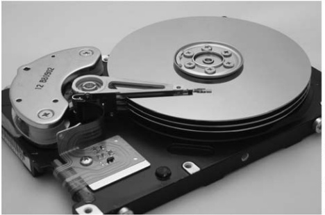
• Disk drive head positioning.
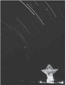
• Antenna pointing for satellites.
• Motor drives in robots and drones.
• Power electronics: DC–DC converter voltage regulation.
• Communication systems: automatic gain control (AGC).

Natural / “biological” control systems

• Blood sugar regulation (pancreas / insulin).
• Heart rate and oxygen delivery in “fight or flight.”
• Eye tracking to keep moving targets centered on the retina.
• Muscle control when you reach and place an object precisely.

Note

Control concepts cut across electrical, mechanical, chemical, biological, and even economic systems.

Underline the universality of feedback and regulation. Ask: “Who wears a smartwatch? It’s measuring your heart rate and sometimes controlling your behavior via notifications. That’s a cyber-physical control loop involving you.”

Case-Study Learning Outcome

We will repeatedly return to a running case study:

Antenna azimuth position control system

You will use it to:

• See how a real electromechanical control loop is built.
• Connect physical hardware (motors, sensors, amplifiers) to block diagrams.
• Visualize transient response, steady-state error, and stability.
• Practice design trade-offs (speed vs. overshoot, accuracy vs. complexity).

Stress that this is not a one-off example; it threads through many chapters. The “antenna azimuth” problem is a classic, but it is also very close to modern applications: gimbals in drones, phased-array pointing, etc.

1.1 Control Systems All Around Us

Control systems are integral to modern society:

• Space shuttle launch and orbit control – rocket thrust, attitude, and trajectory.
• CNC machining – precise movement of tools with cooling and speed control.
• Automated guided vehicles in factories – follow paths and avoid obstacles.

Natural examples inside your body:

• Hormonal control (e.g., insulin) maintains blood sugar.
• Adrenaline raises heart rate and breathing when stressed.
• Eyes and hands coordinate to track and grasp objects.

Even abstract systems like student performance vs. study time can be modeled as control systems.

Use the study-time model as a fun analogy: - Input: study time. - Output: grade. - Disturbance: surprise extra chapter on the exam. - Control action: adjust study plan.

The point is not that the model is perfect, but that control thinking is pervasive.

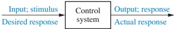
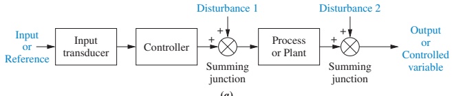
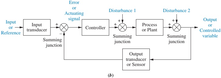
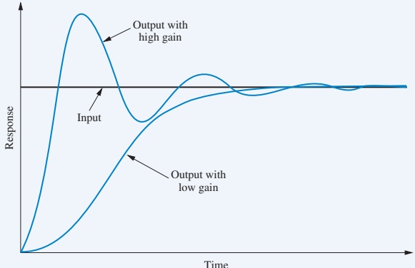
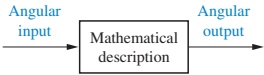
Control System Definition & Basic Block Diagram

Figure 1.1 Simplified description of a control system

A control system consists of:

• Controller – implements the control law.
• Plant / process – physical system we’re controlling.
• Input – desired plant output (command).
• Output – measured plant response.

Relate Figure 1.1 to the previous generic block diagram. Emphasize: here, input is a desired output (e.g., desired elevator floor). Set up that later we will add feedback explicitly to this simple picture.

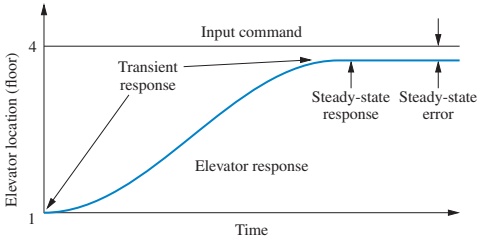
Elevator Example: Input, Output, Performance

• You press the 4th floor button on the 1st floor.
• The car should move:
  • Fast enough (but not scary).
  • Smoothly, without oscillations.
  • Stop level with the floor.

Input: “Go to 4th floor” (a step in desired position).

Output: actual car position vs. time.

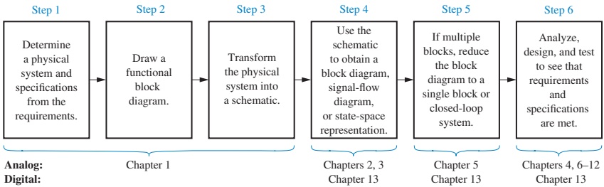
Figure 1.2 Elevator response

Two key performance aspects visible here:

1. Transient response – how the elevator moves while changing floors.
2. Steady-state error – how close the final position is to the floor.

Use the plot conceptually, even if students cannot read all details yet. - Transient response → passenger comfort and patience. - Steady-state error → safety and convenience.

Ask: “Have you ever felt an elevator ‘bounce’ a little at a floor?” That’s underdamped transient behavior.

Why Use Control Systems?

We build control systems to:

1. Amplify power – small electrical signals command large mechanical power.
2. Enable remote control – operate systems from a distance or hazardous area.
3. Change input form – e.g., a knob position → room temperature.
4. Compensate for disturbances – maintain performance despite wind, load changes, noise, etc.

Use the elevator photos:

• Early elevators: human operator pulls ropes, directly controlling motion.
• Modern elevators: motors provide power, control systems manage position and speed.

Emphasize that with control systems, a low-power, convenient command (button press) can safely control a high-power system.

Disturbances & Compensation: Antenna Example

Example: Antenna pointing system

• Goal: keep antenna aimed at a satellite.
• Disturbances:
  • Wind gusts push the antenna off target.
  • Mechanical friction or backlash.
  • Electrical noise in sensors/actuators.

A good control system:

• Detects deviation from commanded angle.
• Applies correction so the antenna returns to the right direction.
• Does this automatically; the reference input does not change.

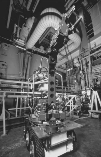
Rover robot arm in contaminated area

Use Rover as another example of remote control in dangerous environments. Link to the antenna case study: we will design such a position loop.

1.2 Brief History of Control Systems (Human-Designed)

Control ideas go back over 2000 years:

• 300 B.C. – Greek water clocks (Ktesibios). Liquid-level regulation to maintain constant flow.
• Ancient oil lamps (Philon of Byzantium). Self-regulated oil level by clever tubing and air pressure.
• 1681 – Papin’s safety valve. Steam pressure regulation via weighted valve.
• 17th century – Drebbel’s incubator. Mechanical temperature controller using alcohol/mercury expansion.

Key theme: automatic regulation of a variable (level, pressure, temperature) using feedback-like mechanisms.

You don’t need students to remember names and dates. Instead, focus on the idea: humans have been building feedback-like devices for centuries. Draw parallels: liquid-level controller → modern tank-level control in chemical plants.

Historical Milestones: Speed Control

• 1745 – Edmund Lee
  • Windmill speed control by automatically changing blade pitch.
• 1809 – William Cubitt
  • Improved windmill with movable louvers for better speed regulation.
• Late 18th century – James Watt’s flyball governor
  • Rotating balls rise with speed, mechanically throttling steam input.
  • Classic mechanical speed feedback system.

Key idea: speed is measured, compared to desired value, and used to adjust input.

Students often have seen animations of Watt’s governor. Make the connection: this is essentially a mechanical proportional feedback controller.

Mathematical Foundations: Stability Criteria

Major contributions in the 19th century:

• Maxwell (1868) – early stability criterion for 3rd-order systems.
• Routh (1874, 1877) – extended criteria to higher orders → Routh–Hurwitz stability test.
• Lyapunov (1892) – generalized stability theory to nonlinear systems.

These works turned practical control problems into mathematical questions about differential equations and their roots.

Tip

In later chapters, you will learn how to decide if a system is stable by looking at coefficients or roots of characteristic equations, not by trial-and-error experiments.

Reassure students: they don’t need to memorize all history, but they should recognize Routh and Lyapunov as names linked to stability methods they will use later.

20th-Century Frequency and Root-Locus Methods

Key developments:

• Nicholas Minorsky (1920s) – theoretical basis of PID control for ship steering.
• Bode & Nyquist (Bell Labs, 1920s–30s) –
  • Feedback amplifier analysis.
  • Bode plots and Nyquist criteria for frequency-domain design.
• Walter R. Evans (1948) –
  • Root locus: graphical method to see how closed-loop poles move as a gain changes.

These are the core analysis tools for classical linear control.

Explain that these methods remain in heavy use in industry and are embedded in tools like MATLAB’s Control System Toolbox. Set expectations: Bode/Nyquist → Chapters 10–11; root locus → Chapters 8–9, 13.

Contemporary Applications

Modern control systems are everywhere:

• Aerospace – missile and spacecraft guidance, aircraft autopilots, UAVs.
• Ships – heading control, roll stabilization, dynamic positioning.
• Process industry – temperature, pressure, concentration, flow, and thickness regulation.
• Automation & robotics – industrial robot arms, collaborative robots, warehouse robots.
• Consumer electronics – camera autofocus, disk drives, optical disk tracking.

Modern systems almost always include a digital computer as part of the controller.

Highlight that ECE graduates will likely interact with digital controllers (microcontrollers, FPGAs, embedded CPUs) implementing control laws.

Space Shuttle: A Complex Control System

The (now retired) space shuttle is a powerful example:

• Onboard computers handled:
  • Navigation – estimating position and velocity from sensors.
  • Guidance – computing desired trajectory and attitude.
  • Control – generating commands to engines, thrusters, and aerosurfaces.
• Control subsystems included:
  • OMS engine gimbaling in space.
  • Elevon and rudder control in atmosphere.
  • Reaction control system (RCS) jets for attitude when aero surfaces were ineffective.
  • Power and life-support regulation (fuel cells, tank pressures, temperatures).

All these formed a hierarchical control architecture.

Use this to convey the scale and complexity of real-world control systems. Make the point that what we study (single-loop position control, etc.) are building blocks in a much larger system-of-systems.

1.3 System Configurations: Open- vs Closed-Loop

Open-loop and closed-loop block diagrams

Closed-loop system

1.3 System Configurations: Open- vs Closed-Loop

Two main architectures:

1. Open-loop systems – no feedback; no automatic correction.
2. Closed-loop (feedback) systems – output is measured and used to adjust input.

Show both figures and verbally identify each block. Stress that in ECE, almost all interesting high-performance controllers are closed-loop; but open-loop still has uses when environment is predictable.

Open-Loop Control: Structure

Characteristics:

• Control signal depends only on the input, not on output.
• Cannot correct for Disturbance 1 (added to controller output) or Disturbance 2 (added at plant output).
• Output may deviate significantly if environment or plant changes.

Give intuitive ECE-style examples: - DSM or microcontroller generating PWM to a heater without temperature feedback. - LED brightness scheduled from a lookup table, not measured. Emphasize: works only if the plant and disturbances are well known and nearly constant.

Open-Loop Examples

• Toaster
  • Input: time setting.
  • Output: toast color.
  • Assumes “longer time → darker toast.”
  • Does not sense actual color, bread type, or thickness.
• Mass–spring–damper with constant force
  • Constant force determines equilibrium position.
  • If another external force (disturbance) is applied, position changes and system does not correct.
• Your study plan
  • You compute hours to study for 3 chapters.
  • Professor adds a 4th chapter (disturbance).
  • If you don’t adjust your plan, you are acting as an open-loop system.

Warning

Open-loop control is simple and cheap, but can be very sensitive to disturbances and modeling errors.

This is a good place to ask students for more open-loop examples. Guide them to think about devices whose operation is purely time-based or schedule-based, with no output measurement.

Closed-Loop (Feedback) Control: Structure

Key features:

• Sensor / output transducer measures output.
• Feedback path returns a signal proportional to output.
• At the summing junction, feedback is subtracted from input to form an error (actuating) signal.
• Controller drives plant to reduce error toward zero.

Explain “unity transducers”: when generation/measurement gains are 1, the actuator signal equals the actual physical error. Emphasize that the system acts to minimize error: if output lags input, error is nonzero, and the controller pushes the plant in the right direction.

Why Feedback Helps

Closed-loop systems:

• Are less sensitive to disturbances and plant parameter variations.
• Can achieve higher accuracy (lower steady-state error).
• Allow designers to shape transient response and steady-state behavior more flexibly by adjusting loop gain or adding compensators.

Trade-offs:

• More complex hardware and software.
• Additional sensors, actuators, and signal processing.
• Potential for instability if the loop is not designed carefully.

Why Feedback Helps

Example: smart toaster oven

• Measures internal light level / humidity → estimates toast “doneness.”
• Adjusts time and heat dynamically.
• More accurate but more complex and costly than a simple timer toaster.

Stress that complexity must be justified by performance gains and application needs. Point ahead: much of this course is about using math to design stable, high-performance feedback loops.

Computer-Controlled Systems

In many modern systems, the controller is a digital computer (microcontroller, DSP, FPGA, etc.).

Advantages:

• Time-sharing: one computer can manage many loops.
• Easy to change controller characteristics via software, not hardware.
• Implement complex algorithms: adaptive control, optimal control, digital filters.
• Perform supervisory tasks: scheduling, fault detection, diagnostics, user interface.

Example: Space Shuttle Main Engine (SSME) controller

• Two digital computers monitored: pressures, temperatures, flows, turbopump speed, valve positions, servo actuators.
• Provided closed-loop control of thrust and mixture ratio.

Connect with students’ embedded systems courses: They’ve likely programmed microcontrollers; here, the difference is the use of feedback on physical variables to meet dynamic performance specs.

1.4 Analysis and Design Objectives

Analysis vs. design:

• Analysis – determine how a given system behaves.
  • Evaluate transient response and steady-state error.
  • Check stability.
• Design – choose or modify system components/parameters to meet performance specs.

Three major objectives for control-system design:

1. Desired transient response.
2. Acceptable steady-state error.
3. Stability.

Other considerations: cost, robustness, hardware constraints.

Tell students that nearly every problem in later chapters will boil down to: “Given a plant and specs on speed, overshoot, error, and stability, design a controller that meets them.”

Transient Response: What Happens Before Steady State?

Transient response = system behavior from the moment the input changes until it settles.

Important because:

• Affects comfort and usability (elevator, car cruise control).
• Affects throughput (disk drive head must settle before reading/writing).
• May affect mechanical stress and reliability (too aggressive motion can damage hardware).

Transient Response: What Happens Before Steady State?

Example: disk drive head

Computer hard disk and head

• Head moves from one track to another.
• Reading/writing cannot start until motion settles.
• Transient performance (speed, overshoot, damping) directly affects transfer rate.

In later chapters we will define metrics like rise time, overshoot, settling time, etc. For now, just convey that transient design is crucial to performance and user experience.

Steady-State Response & Error

Steady-state response = behavior after transients have effectively died out.

Steady-state error (SSE) = difference between desired output and actual output in steady state.

Examples:

• Elevator leveling error: a few centimeters off can be dangerous.
• Antenna tracking error: if too large, satellite falls outside the beam.
• Disk drive head offset: results in read/write errors.

Design goals:

• SSE must be small enough to meet accuracy and safety requirements.
• But sometimes we trade between transient performance and SSE.

Important

Later we will quantify SSE for standard input types (step, ramp, parabola) and relate it to system type and gain.

Emphasize that SSE depends on both system structure (e.g., integrator presence) and loop gain. This foreshadows integral control and error constants.

Stability: The Non-Negotiable Requirement

Total response = natural response + forced response

\[ \text{Total response} = \text{Natural response} + \text{Forced response} \]

• Natural response – how the system behaves due to its own dynamics (homogeneous solution).
• Forced response – driven directly by the input (particular solution).

A useful control system must have a natural response that:

1. Decays to zero as time → ∞, or
2. Oscillates with bounded amplitude.

If the natural response grows without bound, the system is unstable:

• Elevator overspeeds and crashes limit stops.
• Aircraft diverges into uncontrollable roll.
• Antenna oscillates with increasing amplitude, hitting mechanical stops.

Warning

If the system is unstable, discussions of transient response and steady-state error are meaningless. Stability is the first checkpoint.

Mention that in many linear systems, we can infer stability directly from pole locations or Routh-Hurwitz tables. Assure students that they’ll learn precise stability tests, but the intuition is: does the system “settle” or “blow up”?

Other Design Considerations

Beyond transient, SSE, and stability, we must consider:

• Hardware constraints
  • Motor torque and speed limits.
  • Sensor accuracy, range, and bandwidth.
  • Actuator saturation and dead zones.
• Cost and manufacturability
  • Component selection vs. budget.
  • Cost per unit for mass-produced products.
• Robustness / Sensitivity
  • Real systems’ parameters change (temperature, aging, wear).
  • A robust design maintains performance despite parameter variations.
  • Sensitivity analysis quantifies how much specs change when parameters change.

Foreshadow that Chapters 7–8 will look at sensitivity and robustness in more mathematical detail. Point out that several mathematically “optimal” designs are rejected in practice because they are too sensitive or fragile.

Case Study: Antenna Azimuth Control

• We want an antenna to rotate (azimuth) to a commanded angle.
• Typical ECE components:
  • Potentiometer for position sensing.
  • Amplifiers for signal and power.
  • DC motor and gears to move the antenna.

This is a position control system, similar in spirit to:

• Robot joint control.
• Camera pan/tilt platforms.
• Radar and satellite dish pointing.

Radio antenna with position control

Tell students that by understanding this one system well, they gain insight applicable to many other systems with similar structure.

Antenna Azimuth System Layout

Goal: output angle \(\theta_o(t)\) tracks input command \(\theta_i(t)\).

Flow (qualitative):

1. Input angle \(\theta_i(t)\) → potentiometer → input voltage.
2. Output angle \(\theta_o(t)\) → feedback potentiometer → feedback voltage.
3. Error = input voltage – feedback voltage.
4. Signal and power amplifiers amplify error to drive DC motor.
5. Motor + load rotate antenna until error ≈ 0.

Walk through both physical layout and block diagram: - Physical: students see actual motor, gears, potentiometers. - Functional: they see how to abstract to blocks.

Emphasize that in steady state (no disturbance), motor stops when input and output match.

Effect of Controller Gain on Response

• With low gain:
  • Motor turns slowly.
  • Response is sluggish; long time to reach final angle.
  • Often no overshoot.
• With high gain:
  • Motor turns faster toward target.
  • May overshoot and oscillate before settling.
  • Can produce damped oscillations (under-damped response).

Steady-state value may still be exactly correct (zero steady-state error) in both cases, but transients differ.

Effect of controller gain on response

Clarify that, for this system type and step input, increasing gain usually reduces steady-state error but can worsen overshoot and oscillations. Point out that later we’ll see “too much gain” eventually causes instability.

Need for More Than Just Gain: Compensators

Sometimes, adjusting only the gain cannot meet both:

• A desired fast, well-damped transient response, and
• A desired small steady-state error.

Solution: use a controller with dynamic behavior, e.g.:

• Add integrators or filters in the controller.
• Implement full PID controllers or lead/lag compensators.
• Possibly add dynamic elements in the feedback path.

These added dynamics are called compensators.

Note

Compensators give us more degrees of freedom to shape both transient and steady-state performance, at the price of more complexity.

Explain that a pure gain can sometimes force a trade-off (overshoot vs SSE). Compensators (e.g., lead, lag, PID) help to break this trade-off in many cases. You don’t need to define specific compensators yet—that comes in later chapters.

1.5 The Control System Design Process

Design process flow

1.5 The Control System Design Process

Typical steps:

1. Transform requirements into a physical system concept.
2. Draw a functional block diagram.
3. Create a schematic with actual components.
4. Develop a mathematical model (differential equations, transfer functions, or state-space).
5. Reduce to an equivalent block diagram (simplify interconnections).
6. Analyze and design to meet performance specs; iterate with testing.

Emphasize that real design is iterative: - If testing (Step 6) fails, you may need to refine the schematic (Step 3) or even revisit requirements (Step 1). Mention that this flow will structure the rest of the course.

Step 1 – From Requirements to Physical System

Requirements might say:

• Antenna must track commands with:
  • Max settling time: e.g., 1 second.
  • Max overshoot: e.g., 10%.
  • Max steady-state error: small fraction of a degree.
• Constraints: weight, size, power, environmental limits.
• Operational needs: remote operation, maintainability.

From these, we propose a physical concept:

• Antenna + gear train + motor + sensors + electronics.

Highlight that interpreting vague or verbal requirements into precise performance specs is a key engineering skill. Explain that at this stage you think qualitatively about architecture, not detailed math.

Step 2 – Functional Block Diagram

We translate the physical idea into functional blocks:

• Input transducer (potentiometer).
• Controller (amplifiers, logic).
• Plant (motor + load).
• Output transducer (feedback potentiometer).

Functional block diagram of antenna system

Stress that block diagrams are about functions and interconnections, not exact component values. They are a bridge between physical understanding and mathematical modeling.

Step 3 – Schematic Diagram

Next, we draw a more detailed electrical / mechanical schematic:

• Show potentiometers, amplifiers, motor, gear train, load inertia, friction.
• Make simplifying assumptions:
  • Potentiometer inertia and friction negligible.
  • Amplifier dynamics much faster than motor → model as pure gain \(K\).
  • DC motor armature inductance small → model with resistance only.

Antenna schematic (simplified)

Explain that we deliberately simplify to get a tractable model, then later verify these approximations via analysis and experimental testing.

Step 4 – Mathematical Model

We use physical laws to derive equations:

• Kirchhoff’s voltage law (KVL) – sum of voltages around any closed loop is zero.
• Kirchhoff’s current law (KCL) – sum of currents at a node is zero.
• Newton’s laws – sum of forces (or torques) equals mass (or inertia) times acceleration.

For many systems, the model is a linear, time-invariant (LTI) differential equation:

\[ \frac{d^{n} c(t)}{dt^{n}} + a_{n-1} \frac{d^{n-1} c(t)}{dt^{n-1}} + \cdots + a_0 c(t) = b_m \frac{d^{m} r(t)}{dt^{m}} + b_{m-1} \frac{d^{m-1} r(t)}{dt^{m-1}} + \cdots + b_0 r(t) \]

Where:

• \(c(t)\) = output, \(r(t)\) = input.
• Coefficients \(a_i, b_j\) are functions of physical parameters.

Step 4 – Mathematical Model

Alternative models:

• Transfer functions (Laplace domain).
• State-space models (first-order vector form).

You don’t need to derive the equation in class here, but do stress: - Linear models are approximations; they’re powerful because they enable analytic design. - Nonlinear or time-varying aspects may be considered later or in simulations.

Step 5 – Block Diagram Reduction

We interconnect subsystem transfer functions to get an overall block diagram.

For the antenna azimuth system, we can reduce the full diagram to an equivalent single block:

Equivalent antenna block diagram

This “big” transfer function describes the relationship between:

• Input: commanded angle \(\Theta_i(s)\).
• Output: antenna angle \(\Theta_o(s)\).

Mention that Chapter 5 will cover formal rules for combining blocks in series, parallel, and feedback to get an equivalent transfer function.

Step 6 – Analyze and Design

Now we:

1. Apply standard test inputs to predict performance:
   • Impulse, step, ramp, parabola, sinusoid.
2. Analyze:
   • Stability.
   • Transient response metrics.
   • Steady-state error.
3. Design / tune:
   • Adjust gains.
   • Add compensators.
   • Possibly revise earlier steps if specs cannot be met.

Step 6 – Analyze and Design

Standard test inputs:

• Impulse \(\delta(t)\) → pure transient characterization, modeling.
• Step \(u(t)\) → transient + steady-state error.
• Ramp \(t u(t)\), parabola \(\frac12 t^2 u(t)\) → steady-state tracking quality.
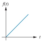
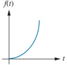
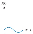
• Sinusoid \(\sin \omega t\) → frequency response and modeling.

Emphasize that these simple inputs are mathematically convenient and still capture key aspects of performance. We often design so these test responses meet specs, which correlates well with performance under more complicated real inputs.

Interactive Exercise – Step Response Intuition

Use this interactive block to explore how gain affects a second-order system’s step response.

viewof wn = Inputs.range([0.1, 10], {step: 0.1, value: 2, label: "Natural frequency ω_n"})
viewof zeta = Inputs.range([0, 2], {step: 0.05, value: 0.4, label: "Damping ratio ζ"})

Ask students to: - Decrease ζ → observe more oscillations and overshoot. - Increase ζ → slower but smoother response. - Increase ωₙ → faster system overall.

Tie this back to the antenna example: gain changes effectively modify these parameters.

1.6 Computer-Aided Design (CAD)

Historically:

• Control design involved hand calculations and manual plotting.
• Large mainframes were needed for complex simulations.

Today:

• Desktop/laptop tools like MATLAB + Control System Toolbox, Simulink, LabVIEW, and others allow:
  • Easy simulation of linear and nonlinear systems.
  • Rapid “what-if” tuning of parameters.
  • Automated plotting of time and frequency responses.
  • Design and optimization of controllers (PID, state feedback, etc.).

Tip

In this course, you should: - First understand the theory and hand calculations. - Then use tools like MATLAB to speed up analysis and explore more complex designs.

Warn students against becoming “button-pushers”: the tools are powerful, but only if they understand what the plots and numbers mean.

1.7 The Control Systems Engineer

A control systems engineer often:

• Works at a system level defining and refining requirements.
• Interfaces with multiple disciplines:
  • Electrical, mechanical, chemical, aerospace, biomedical.
  • Computer science / software, applied mathematics, physics.
• Engages in top-down design:
  • Start with system-level goals and constraints.
  • Break them down into subsystems and detailed designs.

Benefits of studying control systems:

• You will see how earlier courses (circuits, signals, mechanics, programming) fit into a unified system design process.
• You learn a common language that bridges different engineering domains.

Reassure students that this course will help them connect many bits of their curriculum into a coherent whole. Encourage them to think of control as a “glue discipline” that makes systems intelligent and robust.

Summary / Key Points

• A control system regulates a plant’s output to follow a desired input, often in the presence of disturbances.
• Control systems are everywhere: elevators, antennas, disk drives, robots, power converters, biological systems, and more.
• There are two main architectures:
  • Open-loop – simple but cannot correct for disturbances.
  • Closed-loop (feedback) – uses output measurement to reduce error and improve robustness.
• Core performance objectives:
  1. Desired transient response.
  2. Small steady-state error.
  3. Guaranteed stability.

Summary / Key Points

• The design process follows an ordered sequence: from requirements → physical concept → functional diagram → schematic → mathematical model → analysis and design.
• Computer tools (MATLAB, Simulink, LabVIEW, etc.) are essential, but must be used with understanding.
• The antenna azimuth position control system provides a concrete case study to illustrate these ideas throughout the course.

Use this slide as a quick recap. Ask students to volunteer one real-world control system they’ve encountered and identify: input, plant, output, feedback (if any).

Formula & Concept Summary

Although this chapter is mostly conceptual, remember these key mathematical ideas and terms:

• Total response decomposition: \[ \text{Total response} = \text{Natural response} + \text{Forced response} \]

• Standard linear differential equation model (LTI system): \[ \frac{d^{n} c(t)}{dt^{n}} + a_{n-1} \frac{d^{n-1} c(t)}{dt^{n-1}} + \cdots + a_0 c(t) = b_m \frac{d^{m} r(t)}{dt^{m}} + b_{m-1} \frac{d^{m-1} r(t)}{dt^{m-1}} + \cdots + b_0 r(t) \]

• Key performance concepts (to be quantified later):

  • Transient response – rise time, overshoot, settling time, damping.
  • Steady-state error – final error for step/ramp/parabola inputs.
  • Stability – whether natural response decays or grows unbounded.

Formula & Concept Summary

• Standard test inputs (Table 1.1):
  • Impulse: \(\delta(t)\).
  • Step: \(u(t)\).
  • Ramp: \(t\,u(t)\).
  • Parabola: \(\frac{1}{2} t^2 u(t)\).
  • Sinusoid: \(\sin \omega t\).

Mention that upcoming chapters will: - Turn these conceptual definitions into precise mathematical metrics. - Show how to derive transfer functions and state-space models from schematics. - Use these formulas to actually design controllers.

Practice Problem (Conceptual)

You press the accelerator pedal in a car to go from 40 km/h to 60 km/h using cruise control.

1. Identify:
   • Input (reference).
   • Plant.
   • Output.
   • Feedback signal.
2. Suppose the cruise control is disabled and you manually hold the pedal at a fixed position.
   • Is this open-loop or closed-loop control?
   • What kind of disturbances might affect your speed?
3. With cruise control enabled, what advantages does closed-loop control give compared to holding the pedal manually?

Use this as in-class discussion or a quiz. Tie answers back to open-loop vs closed-loop, disturbance rejection, and driver as a (slow, imprecise) feedback element vs electronic controller.

Next Steps

In the next chapter, we will:

• Learn how to derive mathematical models (transfer functions, state-space) from electrical and mechanical schematics.
• Start connecting physical parameters (mass, resistance, inductance, gain) to dynamic behavior.
• Apply these techniques to the antenna azimuth case study.

Encouraged preparation:

• Review basic differential equations (homogeneous + particular solutions).
• Review Laplace transforms and linear time-invariant systems if you’ve seen them.

End by setting expectations: some math is coming, but it will be grounded in physical systems like the antenna. Remind students that the conceptual picture from this chapter should guide their understanding of all the upcoming technical details.